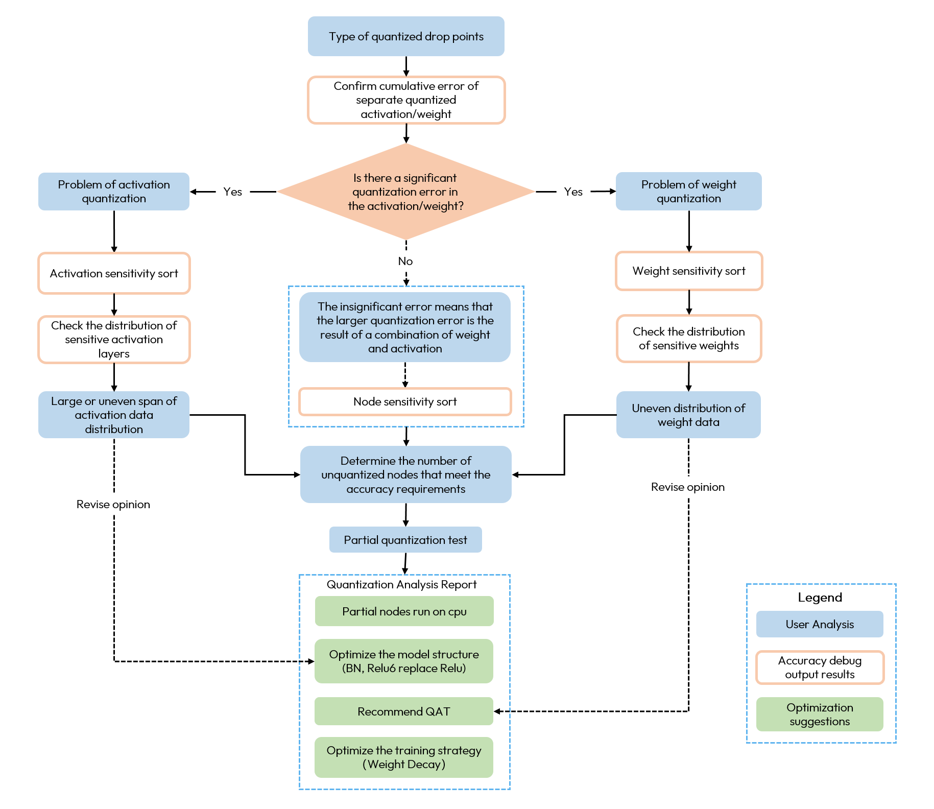
The model conversion toolchain will quantize the calibration of the model based on the calibration samples you provide and guarantee efficient deployment of the model on the Horizon computing platform.
In the process of model conversion, accuracy loss is inevitably introduced due to the quantization process from floating point to fixed point. Usually, the main reasons for accuracy loss may be the following:
A part of the nodes in the model is more sensitive to quantizationwill introduce larger errors, i.e., sensitive node quantization problem.
The error cumulation of each node in the model leads to a large calibration error in the model as a whole, which mainly contains: error cumulation caused by weight quantization, error cumulation caused by activation quantization and error cumulation caused by full quantization.
In this case, Horizon provides the accuracy debug tool to help you locate accuracy problems in the model quantization process on your own.
The tool can help you to analyze the node-granularity quantization error of the calibration model, and finally help you to quickly locate the nodes with accuracy anomalies.
The accuracy debug tool provides a variety of analysis functions for you to use, such as:
Get the node quantization sensitivity.
Get the cumulative error curve of the model.
Get the data distribution of the specified node.
Get the box plot of data distribution between input data channels of a specified node, etc.
First you need to configure debug_mode: "dump_calibration_data" in the yaml file to enable the accuracy debug function.
Save the calibration data (calibration_data), and the related calibration model(calibrated_model.onnx) is saved in a constant state. In which:
Calibration data (calibration_data): In the calibration phase, the model obtains the quantization parameters of each quantized node by forward inference on these data, including: scale and threshold.
Calibration model (calibrated_model.onnx): the quantization parameters of each quantized node calculated in the calibration phase are saved in the calibration node to obtain the calibration model.
Note
What is the difference between the calibration data saved here and the calibration data generated by 02_preprocess.sh?
In J6 toolchain, 02_preprocess.sh gets the same calibration data as the one saved here, both in .npy format, which can be used directly in the debug tool to test the model accuracy. Note that you need to make sure that the folder structure of the calibration data from 02_preprocess.sh is the same as the folder structure of the calibration data saved here before feeding it into the debug tool.
Note
Calibration model (calibrated_model.onnx) interpretation
The calibration model is an intermediate product obtained by the model conversion toolchain by taking the floating point model after structural optimization, calculating the quantization parameters corresponding to each node from the calibration data and saving them in the calibration node.
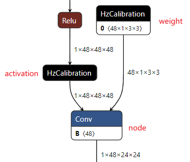
The main feature of the calibration model is that the model contains calibration nodes with the node type HzCalibration.
These calibration nodes are divided into two main categories: activation calibration nodes and weight calibration nodes .
The input of activation calibration node is the output of the previous node of the current node, and the input data is quantized and inverse quantized based on the quantization parameters (scales and thresholds) saved in the current activation calibration node and then output.
The input of weight calibration node is the original floating point weights of the model, and the input original floating point weights are quantized and inverse quantized based on the quantization parameters (scales and thresholds) saved in the current weight calibration node and then output.
In addition to the above calibration nodes, other nodes in the calibration model are called general nodes by the accuracy debug tool. The types of general nodes are: Conv, Mul, Add, etc.
The folder structure of calibration_data is as follows:
|--calibration_data : calibration data|----input.1 : folder named input node of the model and save the corresponding input data|--------0.npy|--------1.npy|-------- ...|----input.2 : for multi-input models multiple folders will be saved|--------0.npy|--------1.npy|-------- ...
Next, you need to import the debug module into your code and get the quantization sensitivity of nodes (by default, the cosine similarity of the model output is used) via the get_sensitivity_of_nodes interface.
A detailed description of the parameters of get_sensitivity_of_nodes can be found in get_sensitivity_of_nodes section.
# Import the debug moduleimport hmct.quantizer.debugger as dbg# Import the log moduleimport logging# If verbose=True, you need to set the log level to INFO first.logging.getLogger().setLevel(logging.INFO)# Get node quantization sensitivitynode_message = dbg.get_sensitivity_of_nodes( model_or_file='./calibrated_model.onnx', metrics=['cosine-similarity', 'mse'], calibrated_data='./calibration_data/', output_node=None, node_type='node', data_num=None, verbose=True, interested_nodes=None)
For customer convenience, the accuracy debug tool can also be used via the command line, which can be viewed via hmct-debugger -h/--help the subcommands corresponding to each function.
The detailed parameters and usage of each subcommand can be found in the Function Description section.
The parameters can be viewed via hmct-debugger get-sensitivity-of-nodes -h/--help.
Parameters:
Parameter
Abbr for Command Line Paramters
Description
Required/Optional
model_or_file
Fixed parameter
PURPOSE: Specify the calibration model. RANGE: None. DEFAULT VALUE: None. DESCRIPTIONS: Required, specify the calibration model to be analyzed.
Required
metrics
-m
PURPOSE: The measure of node quantification sensitivity. RANGE: 'cosine-similarity' , 'mse' , 'mae' , 'mre' , 'sqnr' , 'chebyshev' . DEFAULT VALUE: 'cosine-similarity'. DESCRIPTIONS: Specify how the node quantization sensitivity is calculated, and this parameter can be a List, i.e., calculating the quantized sensitivities in a variety of ways. However, the output is sorted by the calculation of the first position in the list only, and the higher the ranking indicates that the error introduced by quantifying that node is greater.
Optional
calibrated_data
Fixed parameter
PURPOSE: Specify the calibration data. RANGE: None. DEFAULT VALUE: None. DESCRIPTIONS: Required, specify the calibration data needed for the analysis.
Required
output_node
-o
PURPOSE: Specify the output node. RANGE: General nodes with corresponding calibration nodes in the calibration model. DEFAULT VALUE: None. DESCRIPTIONS: This parameter allows you to specify intermediate nodes as output and calculate the node quantization sensitivity.If the default parameter None is kept, the accuracy debug tool will obtain the final output of the model and calculate the quantization sensitivity of the nodes on this basis.
Optional
node_type
-n
PURPOSE: The node type. RANGE: 'node' , 'weight' , 'activation'. DEFAULT VALUE: 'node'. DESCRIPTIONS: The types of nodes that need to calculate the quantization sensitivity, including: node (general node), weight (weight calibration node), activation (activation calibration node).
Optional
data_num
-d
PURPOSE: The amount of data needed to calculate the quantized sensitivities. RANGE: Greater than 0, less than or equal to the total number of data in calibration_data. DEFAULT VALUE: 1. DESCRIPTIONS: Set the amount of data needed to calculate the node quantization sensitivity. The default is 1, in which case the tool will use the first single data in the calibration_data set for the calculation. The minimum setting is 1 and the maximum is the amount of data in calibration_data.
Optional
verbose
-v
PURPOSE: Select whether to print the information to the terminal. RANGE: True , False. DEFAULT VALUE: False. DESCRIPTIONS: If set to True, the quantization sensitivity information will be printed to the terminal. If the metrics contain multiple metrics, they will be sorted by first.
Optional
interested_nodes
-i
PURPOSE: Set the node of interest. RANGE: All nodes in the calibration model. DEFAULT VALUE: None. DESCRIPTIONS: If specified, only the quantization sensitivity of the node will be obtained, and the rest of the nodes will not be obtained. Also, if this parameter is specified, the node type specified by node_type will be ignored. That is, this parameter has a higher priority than node_type. If the default parameter None is kept, the quantization sensitivity of all quantizable nodes in the model is calculated.
Optional
save_dir
-s
PURPOSE: The save path. RANGE: None. DEFAULT VALUE: None. DESCRIPTIONS: Optional, specify the path to save the analysis results.
Optional
API Usage:
# Import the debug moduleimport hmct.quantizer.debugger as dbg# Import the log moduleimport logging# If verbose=True, you need to set the log level to INFO first.logging.getLogger().setLevel(logging.INFO)# Obtain node quantization sensitivitynode_message = dbg.get_sensitivity_of_nodes( model_or_file='./calibrated_model.onnx', metrics=['cosine-similarity', 'mse'], calibrated_data='./calibration_data/', output_node=None, node_type='node', data_num=None, verbose=True, interested_nodes=None)
Description: First you set the node types that need to calculate the sensitivity by node_type, then the tool obtains all the nodes in the calibration model that match node_type and gets the quantization sensitivity of these nodes.
When verbose is set to True, the tool sorts the node quantization sensitivity and prints it in the terminal.
The higher the sort, the greater the quantization error introduced by the node quantization. Also for different node_types, the tool will display different node quantization sensitivity information.
When verbose=True and node_type='node', the following results are printed:
node: The common node after the activation calibration node in the model structure, i.e., the output of the activation calibration node is its input.
threshold: The calibration threshold, and the maximum value is taken if there are multiple thresholds.
bit: The quantization bit.
cosine-similarity, mse: The quantization sensitivity values of each node.
API return value:
The API returns the value of the quantization sensitivity saved in dictionary format (Key is the node name, Value is the quantization sensitivity information of the node), in the following format:
Function: Only one node in the floating-point model will be quantized, and the error of that model and the output of the node in the floating-point model will be calculated sequentially to obtain the cumulative error curve.
The parameters can be viewed via hmct-debugger plot-acc-error -h/--help.
API parameters:
Parameter
Abbr for Command Line Paramters
Description
Required/Optional
save_dir
-s
PURPOSE: The save path. RANGE: None. DEFAULT VALUE: None. DESCRIPTIONS: Optional, specify the path to save the analysis results.
Optional
calibrated_data
Fixed parameter
PURPOSE: Specify the calibration data. RANGE: None. DEFAULT VALUE: None. DESCRIPTIONS: Required, specify the calibration data to be analyzed.
Required
model_or_file
Fixed parameter
PURPOSE: Specify the calibration model. RANGE: None. DEFAULT VALUE: None. DESCRIPTIONS: Required, specify the calibration model to be analyzed.
Required
quantize_node
-q
PURPOSE: Quantize only the specified nodes in the model and view the error accumulation curve. RANGE: All nodes in the calibration model. DEFAULT VALUE: None. DESCRIPTIONS: Optional parameter. Specifies the nodes in the model that need to be quantized, while ensuring that none of the remaining nodes are quantized. It is determined whether the parameter is a nested list to decide whether to quantize a single node or a partial node.
For example:
quantize_node=['Conv_2','Conv_9']: Quantize only Conv_2 and Conv_9, respectively, while ensuring that the remaining nodes are not quantized.
quantize_node=[['Conv_2'],['Conv_9','Conv_2']]: Only Conv_2 and both Conv_2 and Conv_9 were quantified to test the model cumulative error separately.
quantize_node contains two special parameters: 'weight' and 'activation'.
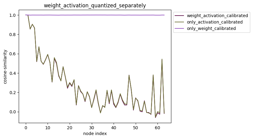
quantize_node = ['weight']: Only quantify weights, not activation.
quantize_node = ['activation']: Only quantify activation, not weights.
quantize_node = ['weight','activation']: Weights and activations are quantified separately.
Note: quantize_node and non_quantize_node cannot be None at the same time, one of them must be specified.
Optional
non_quantize_node
-nq
PURPOSE: Specify the node in the unquantized model to view the error accumulation curve. RANGE: All nodes in the calibration model. DEFAULT VALUE: None. DESCRIPTIONS: Optional parameter. Specifies the nodes in the model that are not quantized, while ensuring that all the remaining nodes are quantized.
This parameter determines whether a single node is unquantized or partially quantized by determining whether it is a nested list.
For example:
non_quantize_node=['Conv_2','Conv_9']: Unquantize the Conv_2 and Conv_9 nodes respectively, while ensuring that all the remaining nodes are quantized.
non_quantize_node=[['Conv_2'],['Conv_9','Conv_2']]: Only Conv_2 quantization and both Conv_2 and Conv_9 quantization are unquantized to test the model cumulative error separately.
Note: quantize_node and non_quantize_node cannot be None at the same time, one of them must be specified.
Optional
metric
-m
PURPOSE: The error metric method. RANGE: 'cosine-similarity', 'mse', 'mae', 'mre', 'sqnr', 'chebyshev'. DEFAULT VALUE: 'cosine-similarity'. DESCRIPTIONS: Set the calculation method for calculating the model error.
Optional
average_mode
-a
PURPOSE: Specify the output mode of the cumulative error curve. RANGE: True ,False. DEFAULT VALUE: False. DESCRIPTIONS: The default is False, if True, then the average of the cumulative error is obtained as the result.
Optional
# Import the debug moduleimport hmct.quantizer.debugger as dbgdbg.plot_acc_error( save_dir: str, calibrated_data: str or CalibrationDataSet, model_or_file: ModelProto or str, quantize_node: List or str, non_quantize_node: List or str, metric: str = 'cosine-similarity', average_mode: bool = False):
Analysis results display:
1. Specify the node to quantify the cumulative error test:
Specify single-node quantization
Configuration method: quantize_node=['Conv_2', 'Conv_90'], quantize_node is single list.
API Usage:
# Import the debug moduleimport hmct.quantizer.debugger as dbgdbg.plot_acc_error( save_dir='./', calibrated_data='./calibration_data/', model_or_file='./calibrated_model.onnx', quantize_node=['Conv_2', 'Conv_90'], metric='cosine-similarity', average_mode=False)
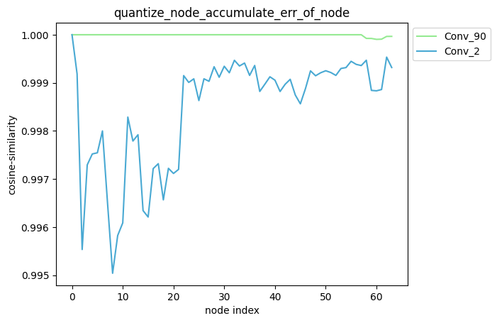
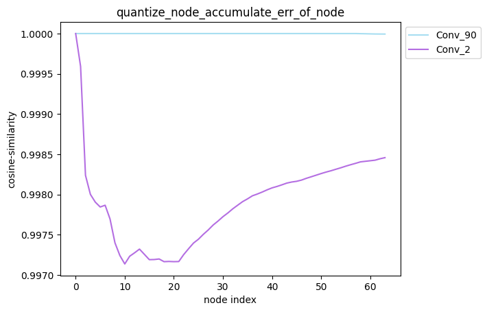
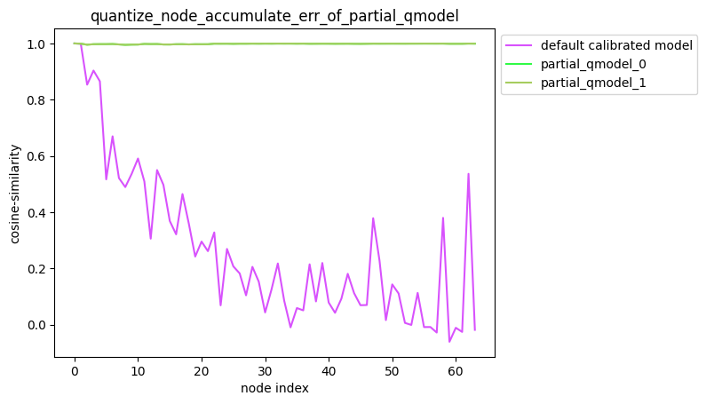
Description: When quantize_node is a single list, for the quantize_node you set, quantize the nodes in the quantize_node separately and keep the other nodes in the model unquantized to get the corresponding model, and then calculate the error between the output of each node in the model and the output of the corresponding node in the floating-point model, and get the corresponding cumulative error curve.
When average_mode = False:
When average_mode = True:
Note
average_mode
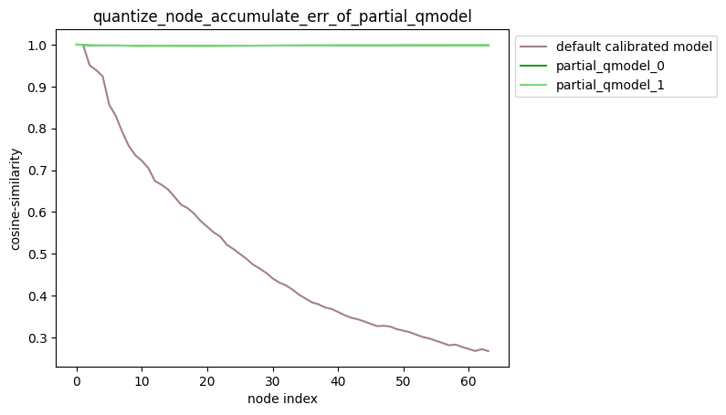
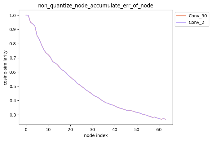
average_mode defaults to False. For some models, it is not possible to determine which quantization strategy is more effective by the cumulative error curve.
Therefore, we need to set average_mode to True, which takes the average value of the cumulative error of the first n nodes as the cumulative error of the nth node.
This is calculated as follows, for example:
When average_mode=False, accumulate_error=[1.0, 0.9, 0.9, 0.8].
But when average_mode=True, accumulate_error=[1.0, 0.95, 0.933, 0.9].
Specify multiple nodes for quantization
Configuration method: quantize_node=[['Conv_2'], ['Conv_2', 'Conv_90']],quantize_node is nested list.
API Usage:
# Import the debug moduleimport hmct.quantizer.debugger as dbgdbg.plot_acc_error( save_dir='./', calibrated_data='./calibration_data/', model_or_file='./calibrated_model.onnx', quantize_node=[['Conv_2'], ['Conv_2', 'Conv_90']], metric='cosine-similarity', average_mode=False)
Description: When quantize_node is a nested list, for the quantize_node you set, quantize the nodes specified for each single list in the quantize_node separately and keep the other nodes in the model unquantized to get the corresponding model,
then calculate the error between the output of each node in the model and the output of the corresponding node in the floating-point model, and get the corresponding cumulative error curve.
partial_qmodel_0: Only quantize the Conv_2 node, the rest of the nodes are not quantized;
partial_qmodel_1: Only the Conv_2 and Conv_90 nodes are quantified, and the rest of the nodes are not quantified.
When average_mode = False:
When average_mode = True:
2.Cumulative error test after unquantizing some nodes of the model
Specify single node not quantified
Configuration method: non_quantize_node=['Conv_2', 'Conv_90'],non_quantize_node is single list.
API Usage:
# Import the debug moduleimport hmct.quantizer.debugger as dbgdbg.plot_acc_error( save_dir='./', calibrated_data='./calibration_data/', model_or_file='./calibrated_model.onnx', non_quantize_node=['Conv_2', 'Conv_90'], metric='cosine-similarity', average_mode=True)
Command Line Usage:
hmct-debugger plot-acc-error calibrated_model.onnx calibration_data -nq ['Conv_2','Conv_90'] -a True
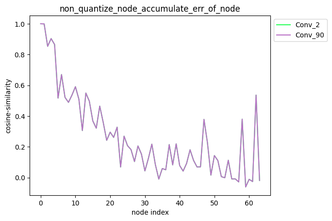
Description: When the non_quantize_node is a single list, for the non_quantize_node you set, unquantize each node in the non_quantize_node separately while keeping all other nodes quantized,
and then get the corresponding model, calculate the error between the output of each node in the model and the output of the corresponding node in the floating-point model, and get the corresponding cumulative error curve.
When average_mode = False:
When average_mode = True:
Specify multiple nodes not to quantize
Configuration method: non_quantize_node=[['Conv_2'], ['Conv_2', 'Conv_90']],non_quantize_node is nested list.
API Usage:
# Import the debug moduleimport hmct.quantizer.debugger as dbgdbg.plot_acc_error( save_dir='./', calibrated_data='./calibration_data/', model_or_file='./calibrated_model.onnx', non_quantize_node=[['Conv_2'], ['Conv_2', 'Conv_90']], metric='cosine-similarity', average_mode=False)
Description: When non_quantize_node is a nested list, for the non_quantize_node you set, do not quantize each node specified in the non_quantize_node and keep all the other nodes in the model quantized,
and get the corresponding model, then calculate the error between the output of each node in the model and the output of the corresponding node in the floating-point model, and get the corresponding cumulative error curve.
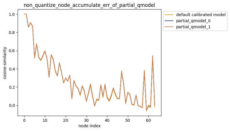
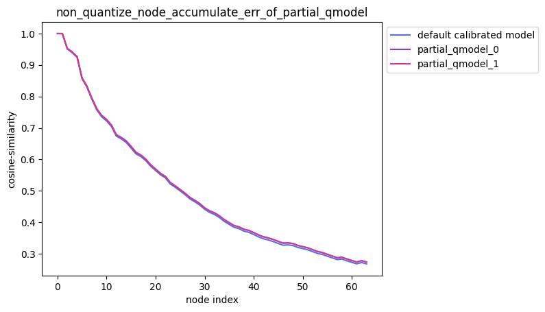
partial_qmodel_0: No quantization of Conv_2 nodes and quantization of the remaining nodes;
partial_qmodel_1: No quantization of Conv_2 and Conv_90 nodes, and quantization of the rest of the nodes.
When average_mode = False:
When average_mode = True:
Test skills:
When testing the accuracy of partial quantification, you may compare the accuracy of multiple sets of quantified strategies in order of quantified sensitivity, in which case you can refer to the following usage:
# Import the debug moduleimport hmct.quantizer.debugger as dbg# First, use the quantization sensitivity sorting function to obtain the quantization sensitivity sorting of the nodes in the modelnode_message = dbg.get_sensitivity_of_nodes( model_or_file='./calibrated_model.onnx', metrics='cosine-similarity', calibrated_data='./calibration_data/', output_node=None, node_type='node', verbose=False, interested_nodes=None)# node_message is a dictionary type, and its key value is the node namenodes = list(node_message.keys())# Specify the unquantized nodes by nodes, which can be easily useddbg.plot_acc_error( save_dir='./', calibrated_data='./calibration_data/', model_or_file='./calibrated_model.onnx', non_quantize_node=[nodes[:1], nodes[:2]], metric='cosine-similarity', average_mode=True)
Description: The quantize_node can also be specified directly as 'weight' or 'activation'.
quantize_node = ['weight']: Quantify weights, not activation.
quantize_node = ['activation']: Quantify activation, not weights.
quantize_node = ['weight', 'activation']: Weights and activations are quantified separately.
Note
In general, it is recommended that you pay more attention to the portion of the cumulative error curve near the model output location in the cumulative error curve graph.
When the cumulative error curve obtained from the test after using a certain quantization method has a smaller cumulative error close to the model output position, i.e.,
a higher degree of similarity, then we recommend that you prioritize testing this quantitative method.
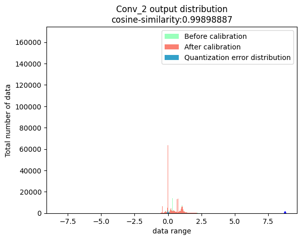
Function:Select the node and obtain the output of that node in the floating point model and the calibration model respectively to get the output data distribution.
In addition, the two outputs are subtracted to obtain the error distribution between the two outputs.
The parameters can be viewed via hmct-debugger plot-distribution -h/--help.
Parameters:
Parameter
Abbr for Command Line Paramters
Description
Required/Optioanl
save_dir
-s
PURPOSE: The save path. RANGE: None. DEFAULT VALUE: None. DESCRIPTIONS: Optional, specify the path to save the analysis results.
Optional
model_or_file
Fixed parameter
PURPOSE: Specify the calibration model. RANGE: None. DEFAULT VALUE: None. DESCRIPTIONS: Required, specify the calibration model to be analyzed.
Required
calibrated_data
Fixed parameter
PURPOSE: Specify the calibration data. RANGE: None. DEFAULT VALUE: None. DESCRIPTIONS: Required, specify the calibration data needed for the analysis.
Required
nodes_list
-n
PURPOSE: Specify the nodes to be analyzed. RANGE: All nodes in the calibration model. DEFAULT VALUE: None. DESCRIPTIONS: Required, specify the nodes to be analyzed. If the node type in nodes_list is:
Weights calibration node: plots the data distribution of the original weights and the weights after calibration.
Activate calibration nodes: Plot the input data distribution of activated calibration nodes.
Common node: Plot the output data distribution of this node before and after quantization, and also plot the error distribution between the two.
Note: nodes_list is a list type, a series of nodes can be specified, and all three types of nodes can be specified at the same time.
Required
# Import the debug moduleimport hmct.quantizer.debugger as dbgdbg.plot_distribution( save_dir: str, model_or_file: ModelProto or str, calibrated_data: str or CalibrationDataSet, nodes_list: List[str] or str)
Analysis results display:
API Usage:
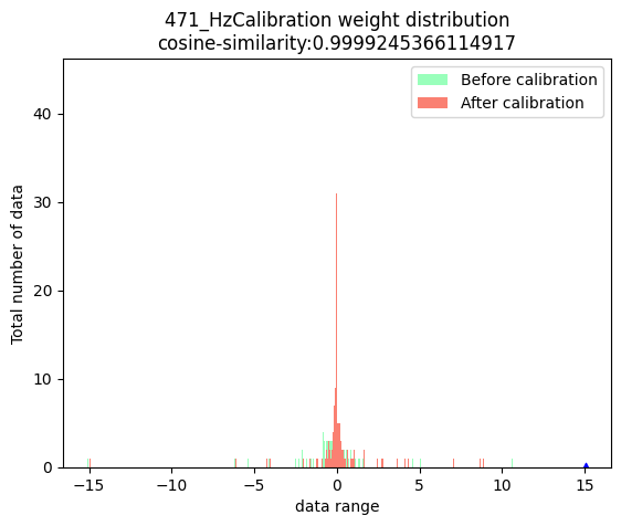
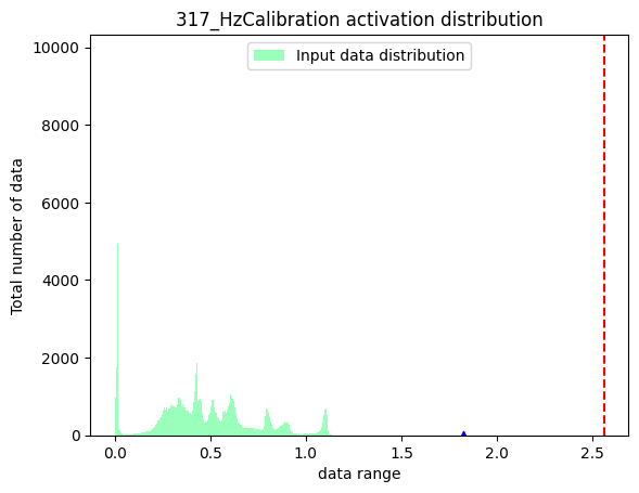
# Import the debug moduleimport hmct.quantizer.debugger as dbgdbg.plot_distribution( save_dir='./', model_or_file='./calibrated_model.onnx', calibrated_data='./calibration_data', nodes_list=['317_HzCalibration', # Activation Node '471_HzCalibration', # Weight Node 'Conv_2']) # Common Node
In the above three pictures, the blue triangle indicates that the maximum value of the absolute data. The red dashed line indicates that the maximum calibration threshold.
The parameters can be viewed via hmct-debugger get-channelwise-data-distribution -h/--help.
Parameters:
Parameter
Abbr for Command Line Paramters
Description
Required/Optioanl
save_dir
-s
PURPOSE: The save path. RANGE: None. DEFAULT VALUE: None. DESCRIPTIONS: Optional, specify the path to save the analysis results.
Optional
model_or_file
Fixed parameter
PURPOSE: Specify the calibration model. RANGE: None. DEFAULT VALUE: None. DESCRIPTIONS: Required, specify the calibration model to be analyzed.
Required
calibrated_data
Fixed parameter
PURPOSE: Specify the calibration data. RANGE: None. DEFAULT VALUE: None. DESCRIPTIONS: Required, specify the calibration data needed for the analysis.
Required
nodes_list
-n
PURPOSE: Specify the calibration node. RANGE: All weight calibration nodes and activation calibration nodes in the calibration model. DEFAULT VALUE: None. DESCRIPTIONS: Required, specify the calibration node.
Required
axis
-a
PURPOSE: Specify the dimension where the channel is located. RANGE: Less than the dimension of node input data. DEFAULT VALUE: None. DESCRIPTIONS: The position of the channel information in the shape. The default parameter is None,
at this time, for the activation calibration node, the second dimension of the node input data is considered to represent the channel information by default,
i.e. axis=1; for the weight calibration node, the axis parameter in the node's attributes will be read as the channel information.
Optional
# Import the debug moduleimport hmct.quantizer.debugger as dbgdbg.get_channelwise_data_distribution( save_dir: str, model_or_file: ModelProto or str, calibrated_data: str or CalibrationDataSet, nodes_list: List[str], axis: int = None)
Analysis results display:
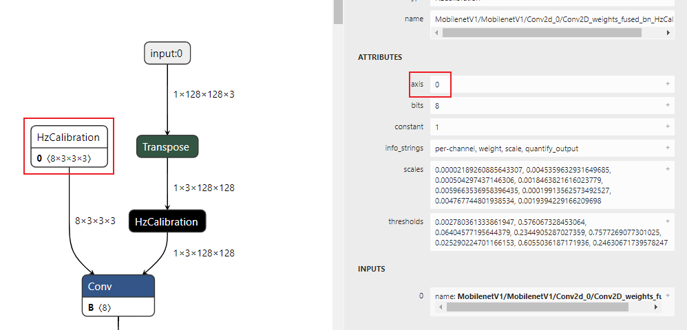
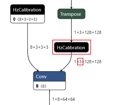
Description: For your set calibration node list(node_list), get the dimension where the channel is located from the parameter axis, and get the data distribution among the node input data channels. Where axis is None by default, if the node is a weight calibration node, then the dimension where the channel is located is 0 by default; if the node is an activation calibration node, then the dimension where the channel is located is 1 by default.
Weight calibration node:
Activation calibration node:
The output is shown as follows:
In the figure:
The horizontal coordinate indicates the number of channels of input data of the node, and there are 96 channels of input data in the figure example.
The vertical coordinate indicates the data distribution range of each channel, where the red solid line indicates the median of the data in that channel and the blue dashed line indicates the mean.
The upper and lower limits of each box indicate the upper quartile and the lower quartile, respectively, and the discrete points outside the upper and lower limits indicate the outliers,
and the maximum of the absolute value of these outliers is observed to determine whether the current node input data is experiencing large fluctuations.
Function: For quantization-sensitive nodes, the model accuracy after quantizing these nodes individually as well as partially is analyzed and tested separately.
The parameters can be viewed via hmct-debugger sensitivity-analysis -h/--help.
Parameters:
Parameter
Abbr for Command Line Paramters
Description
Required/Optioanl
model_or_file
Fixed parameter
PURPOSE: Specify the calibration model. RANGE: None. DEFAULT VALUE: None. DESCRIPTIONS: Required, specify the calibration model to be analyzed.
Required
calibrated_data
Fixed parameter
PURPOSE: Specify the calibration data. RANGE: None. DEFAULT VALUE: None. DESCRIPTIONS: Required, specify the calibration data needed for the analysis.
Required
pick_threshold
-p
PURPOSE: Setting the sensitivity threshold for selected nodes. RANGE: None. DEFAULT VALUE: 0.999. DESCRIPTIONS: Optional parameter. This function calculates the quantitative sensitivity of common nodes and selects nodes with sensitivity less than pick_threshold as sensitive nodes for analysis and testing.
Note: When sensitive_nodes is set, the sensitive_nodes will be tested directly, without calculating node sensitivity and selecting sensitive nodes according to pick_threshold.
Optional
data_num
-d
PURPOSE: Amount of data needed to calculate quantitative sensitivity. RANGE: Greater than 0, less than or equal to the total number of data in calibration_data. DEFAULT VALUE: 1. DESCRIPTIONS: Set the amount of data needed to calculate the node quantization sensitivity.
Optional
sensitive_nodes
-sn
PURPOSE: Specify the sensitive nodes to be analyzed. RANGE: All nodes in the calibration model. DEFAULT VALUE: None. DESCRIPTIONS: Optional, specify the sensitive nodes to be analyzed.
Note: When this parameter is set, the nodes in this parameter are tested directly without calculating the node sensitivity and selecting sensitive nodes based on pick_threshold.
Optional
qtype
-q
PURPOSE: the target qtype for sensitive nodes. RANGE: float32, int16, int8. DEFAULT VALUE: float32. DESCRIPTIONS: Optional, specify the target qtype for sensitive nodes.
Optional
save_dir
-sd
PURPOSE: Save Path. RANGE: None. DEFAULT VALUE: None. DESCRIPTIONS: Optional, specifies the path where the analysis results are saved.
Optional
API Usage:
import hmct.quantizer.debugger as dbgdbg.sensitivity_analysis(model_or_file='calibrated_model.onnx', calibrated_data='calibration_data', pick_threshold=0.9999, data_num=1, qtype="float32", sensitive_nodes=[])
original_qtype, original: The original quantization type of the node, and the output similarity between the float model and the model where all previous (excluding the current) sensitive nodes have their quantization types set to the target qtype.
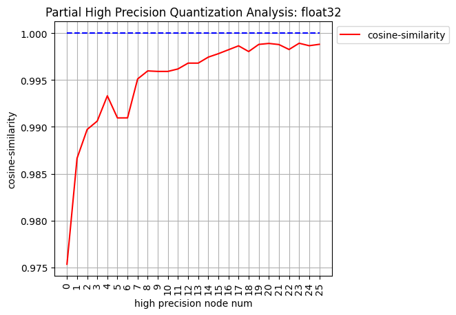
improved_qtype, improved: The qtype assigned to the node, and the output similarity between the float model and the model where this node and all preceding nodes have their quantization types set to the target qtype.
In the figure:
Blue dashed line: similarity between the float model's output and its own output.
Red solid line: similarity between the float model's output and the output of the model where the current node and all preceding nodes are set to the target qtype. For example, in the figure above, setting the top three most sensitive nodes — 'Conv_2', 'Conv_90', and 'Conv_77' — to float32 can restore the model's output similarity to around 0.99.
Note
The point at x = 0 in the figure represents the output similarity of the calibrated model.
The parameters can be viewed via hmct-debugger runall -h/--help.
Parameters:
Parameter
Abbr for Command Line Paramters
Description
Required/Optioanl
model_or_file
Fix parameter
PURPOSE: Specify the calibration model. RANGE: None. DEFAULT VALUE: None. DESCRIPTIONS: Required, specify the calibration model to be analyzed.
Required
calibrated_data
Fix parameter
PURPOSE: Specify the calibration data. RANGE: None. DEFAULT VALUE: None. DESCRIPTIONS: Required, specify the calibration data needed for the analysis.
Required
save_dir
-s
PURPOSE: The save path. RANGE: None. DEFAULT VALUE: None. DESCRIPTIONS: Specify the path to save the analysis results.
Optional
ns_metrics
-nm
PURPOSE: The measure of node quantification sensitivity. RANGE: 'cosine-similarity', 'mse', 'mae', 'mre', 'sqnr', 'chebyshev'. DEFAULT VALUE: 'cosine-similarity'. DESCRIPTIONS: Specify how the node quantization sensitivity is calculated, and this parameter can be a List,
i.e., calculating the quantized sensitivities in a variety of ways. However, the output is sorted by the calculation of the first position in the list only,
and the higher the ranking indicates that the error introduced by quantifying that node is greater.
Optional
output_node
-o
PURPOSE: Specify the output node. RANGE:General nodes with corresponding calibration nodes in the calibration model. DEFAULT VALUE: None. DESCRIPTIONS: This parameter allows you to specify intermediate nodes as output and calculate the node quantization sensitivity.
If the default parameter None is kept, the accuracy debug tool will obtain the final output of the model and calculate the quantization sensitivity of the nodes on this basis.
Optional
node_type
-nt
PURPOSE: The node type. RANGE: 'node', 'weight'. DEFAULT VALUE: 'node'. DESCRIPTIONS: The types of nodes that need to calculate the quantization sensitivity, including: node (general node),
weight (weight calibration node), activation (activation calibration node).
Optional
data_num
-dn
PURPOSE: The amount of data needed to calculate the quantized sensitivities. RANGE: Greater than 0, less than or equal to the total number of data in calibration_data. DEFAULT VALUE: None. DESCRIPTIONS: Set the amount of data needed to calculate the node quantization sensitivity.
The default is None, in which case the tool will default to using all the data in calibration_data for the calculation.
The minimum setting is 1 and the maximum is the amount of data in calibration_data.
Optional
verbose
-v
PURPOSE: Select whether to print the information to the terminal. RANGE: True, False. DEFAULT VALUE: False. DESCRIPTIONS: If set to True, the quantization sensitivity information will be printed to the terminal.
If the metrics contain multiple metrics, they will be sorted by first.
Optional
interested_nodes
-i
PURPOSE: Set the node of interest. RANGE: All nodes in the calibration model. DEFAULT VALUE: None. DESCRIPTIONS: If specified, only the quantization sensitivity of the node will be obtained, and the rest of the nodes will not be obtained.
Also, if this parameter is specified, the node type specified by node_type will be ignored.
That is, this parameter has a higher priority than node_type.
If the default parameter None is kept, the quantization sensitivity of all quantizable nodes in the model is calculated.
Optional
dis_nodes_list
-dnl
PURPOSE: Specify the nodes to be analyzed. RANGE: All nodes in the calibration model. DEFAULT VALUE: None. DESCRIPTIONS: Specify the nodes to be analyzed. If the node type in nodes_list is:
Weights calibration node: plots the data distribution of the original weights and the weights after calibration.
Activate calibration nodes: Plot the input data distribution of activated calibration nodes.
Common node: Plot the output data distribution of this node before and after quantization, and also plot the error distribution between the two.
Note: nodes_list is a list type, a series of nodes can be specified, and all three types of nodes can be specified at the same time.
Optional
cw_nodes_list
-cn
PURPOSE: Specify the calibration node. RANGE: All weight calibration nodes and activation calibration nodes in the calibration model. DEFAULT VALUE: None. DESCRIPTIONS: Specify the calibration node.
Optional
axis
-a
PURPOSE: Specify the dimension where the channel is located. RANGE: Less than the dimension of node input data. DEFAULT VALUE: None. DESCRIPTIONS: The position of the channel information in the shape. The default parameter is None ,
at this time, for the activation calibration node, the second dimension of the node input data is considered to represent the channel information by default, i.e. axis=1;
for the weight calibration node, the axis parameter in the node's attributes will be read as the channel information.
optional
quantize_node
-qn
PURPOSE: Quantize only the specified nodes in the model and view the error accumulation curve. RANGE: All nodes in the calibration model. DEFAULT VALUE: None. DESCRIPTIONS: Optional parameter. Specifies the nodes in the model that need to be quantized, while ensuring that none of the remaining nodes are quantized.
It is determined whether the parameter is a nested list to decide whether to quantize a single node or a partial node.
For example:
quantize_node=['Conv_2', 'Conv_9']: Quantize only Conv_2 and Conv_9, respectively, while ensuring that the remaining nodes are not quantized.
quantize_node=[['Conv_2'], ['Conv_9', 'Conv_2']]: Only Conv_2 and both Conv_2 and Conv_9 were quantified to test the model cumulative error separately.
quantize_node contains two special parameters: 'weight' and 'activation'.
quantize_node = ['weight']: Only quantify weights, not activation.
quantize_node = ['activation']: Only quantify activation, not weights.
quantize_node = ['weight', 'activation']: Weights and activations are quantified separately.
Note: quantize_node and non_quantize_node cannot be None at the same time, one of them must be specified.
Optional
non_quantize_node
-nqn
PURPOSE: Specify the node in the unquantized model to view the error accumulation curve. RANGE: All nodes in the calibration model. DEFAULT VALUE: None. DESCRIPTIONS: Optional parameter. Specifies the nodes in the model that are not quantized, while ensuring that all the remaining nodes are quantized.
This parameter determines whether a single node is unquantized or partially quantized by determining whether it is a nested list.
For example:
non_quantize_node=['Conv_2', 'Conv_9']: Unquantize the Conv_2 and Conv_9 nodes respectively, while ensuring that all the remaining nodes are quantized
non_quantize_node=[['Conv_2'], ['Conv_9', 'Conv_2']]: Only Conv_2 quantization and both Conv_2 and Conv_9 quantization are unquantized to test the model cumulative error separately.
Note: quantize_node and non_quantize_node cannot be None at the same time, one of them must be specified.
Optional
ae_metric
-am
PURPOSE: The error metric method. RANGE: 'cosine-similarity', 'mse', 'mae', 'mre', 'sqnr', 'chebyshev'. DEFAULT VALUE: 'cosine-similarity'. DESCRIPTIONS: Set the calculation method for calculating the model error.
Optional
average_mode
-avm
PURPOSE: Specify the output mode of the cumulative error curve. RANGE: True, False. DEFAULT VALUE: False. DESCRIPTIONS: The default is False, if True, then the average of the cumulative error is obtained as the result.
Optional
pick_threshold
-pt
PURPOSE: Setting the sensitivity threshold for selected nodes. RANGE: None. DEFAULT VALUE: 0.999. DESCRIPTIONS: Optional parameter. This function calculates the quantitative sensitivity of common nodes and selects nodes with sensitivity less than pick_threshold as sensitive nodes for analysis and testing.
Note: When sensitive_nodes is set, the sensitive_nodes will be tested directly, without calculating node sensitivity and selecting sensitive nodes according to pick_threshold.
Optional
sensitive_nodes
-sn
PURPOSE: Specify the sensitive nodes to be analyzed. RANGE: All nodes in the calibration model. DEFAULT VALUE: None. DESCRIPTIONS: Optional, specify the sensitive nodes to be analyzed.
Note: When this parameter is set, the nodes in this parameter are tested directly without calculating the node sensitivity and selecting sensitive nodes based on pick_threshold.
Optional
API Usage:
# 导入debug模块import hmct.quantizer.debugger as dbgdbg.runall(model_or_file='calibrated_model.onnx', calibrated_data='calibration_data')
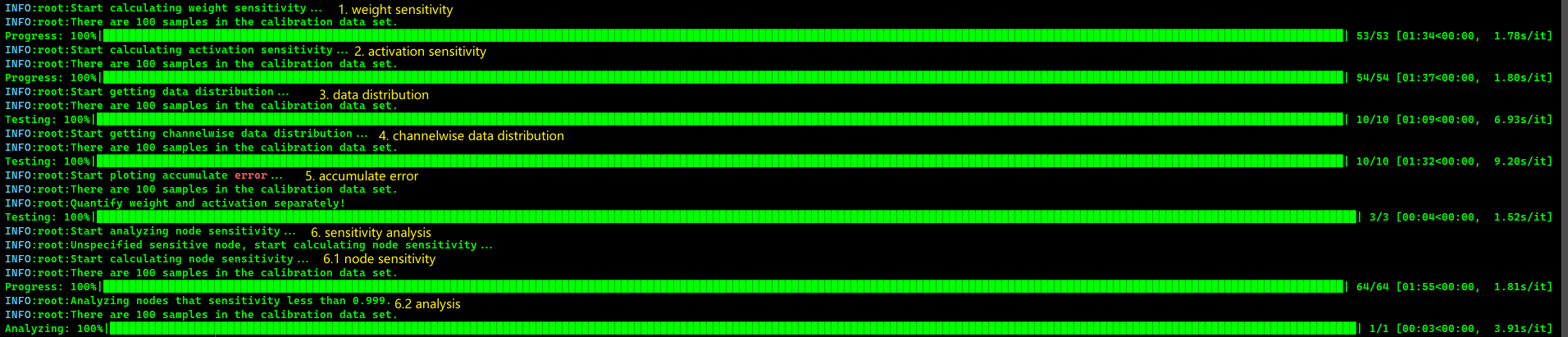
When all parameters are left as default, the tool performs the following functions in sequence:
STEP1 and STEP2: Obtain the quantization sensitivity of the weight calibration node and activation calibration node, respectively.
STEP3: Based on the results of STEP1 and STEP2, take the TOP5 of the weight calibration nodes and the TOP5 of the activation calibration nodes to plot their data distribution, respectively.
STEP4: For the nodes obtained in STEP3, draw box-and-line plots of their inter-channel data distribution, respectively.
STEP5: Plot the cumulative error curves for quantizing only the weights and only the activations, respectively.
STEP6: Partial quantization and single-node quantization accuracy analysis for sensitive nodes.
Since the example in the figure does not specify sensitive_nodes, the debug tool needs to calculate the quantization sensitivity of common nodes by itself and select nodes with sensitivity less than the specified pick_threshold for testing and analysis.
When node_type='node' is specified, the tool will get the top5 nodes and find the calibration nodes corresponding to each node separately, and get the data distribution and box line diagram of the calibration nodes.