PyTorch Model Quick Start

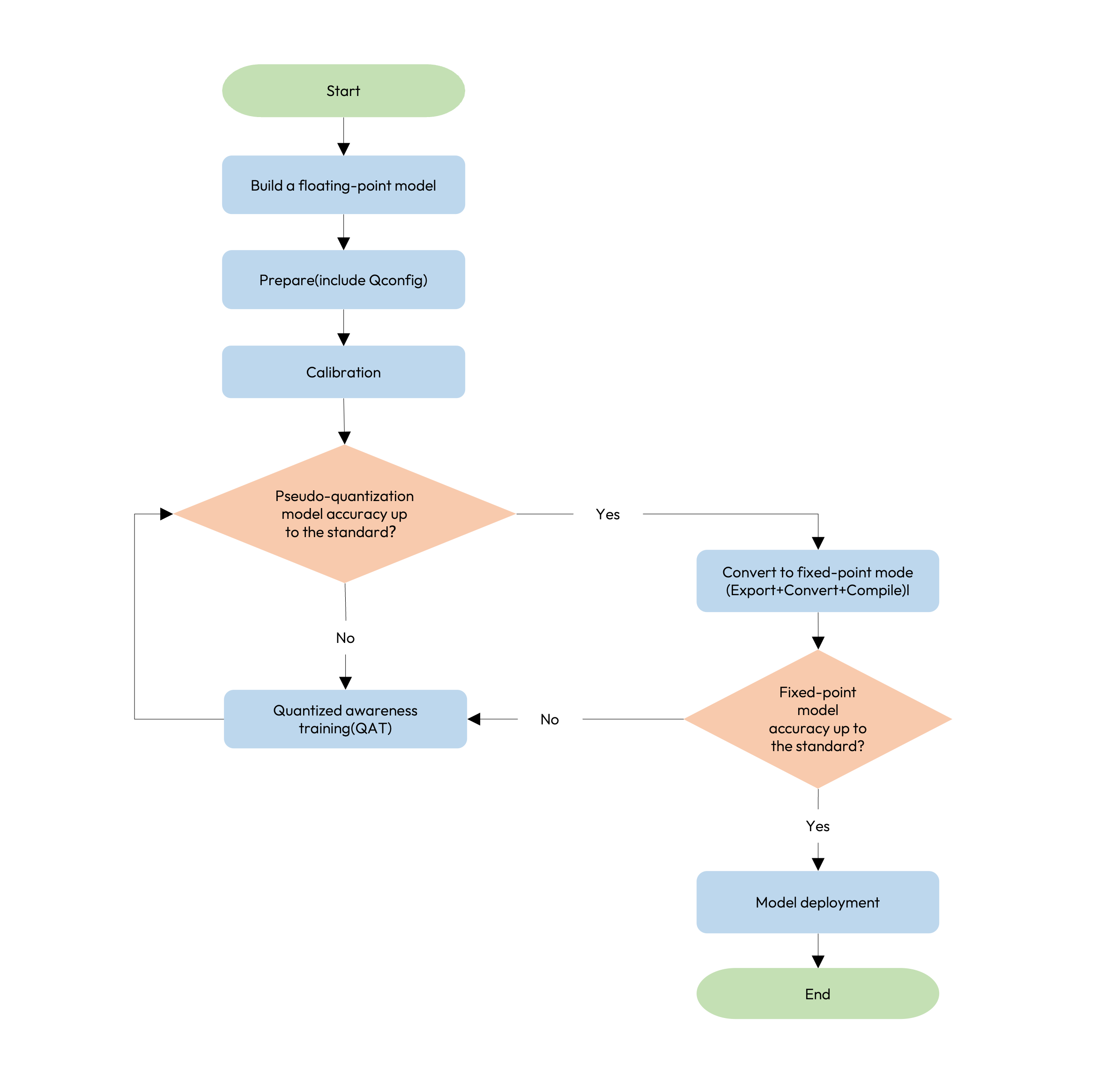
In this chapter, we use the MobileNetV2 model in torchvision as an example to introduce the basic workflow of a PyTorch model from floating-point model adaptation, Calibration, HBIR export, fixed-point model verification, to board deployment, so that you can first run through a minimal end-to-end path.

Attention

Before you start, make sure that the development environment on both the dev PC and the dev board has been prepared, and that PyTorch, horizon_plugin_pytorch, hbdk4, and the related toolchain dependencies are available in the current environment.

To keep the end-to-end process concise, this example uses the CIFAR-10 dataset instead of ImageNet-1K.

Before you start, create a Python example file on the dev PC, for example quick_start_mobilenetv2.py. The Python code below can be added to this file in order and run on the dev PC by executing python3 quick_start_mobilenetv2.py.

Basic Preparation

The following example directly uses torchvision.models.MobileNetV2 to build the floating-point model, and inserts QuantStub before the model input and DeQuantStub after the model output, so that the model has the basic structure required for later quantization and deployment.

Import Dependencies

These dependencies cover the core modules required for data preparation, quantization preparation, HBIR export, and compilation. The code in the following sections is based on these imports.

First, add the following code to the beginning of quick_start_mobilenetv2.py.

import os
from typing import Callable, List, Optional, Tuple

import numpy as np
import torch
import torch.nn as nn
import torchvision.transforms as transforms
from torch import Tensor
from torch.quantization import DeQuantStub
from torch.utils import data
from torchvision.datasets import CIFAR10
from torchvision.models.mobilenetv2 import MobileNetV2

from horizon_plugin_pytorch.functional import rgb2centered_yuv
from horizon_plugin_pytorch.march import set_march
from horizon_plugin_pytorch.quantization import (
    FakeQuantState,
    PrepareMethod,
    QuantStub,
    get_qconfig,
    prepare,
    set_fake_quantize,
)
from horizon_plugin_pytorch.quantization.hbdk4 import export
from horizon_plugin_pytorch.quantization.qconfig_setter import *
from hbdk4 import compiler as hb4
from hbdk4.compiler import save

Basic Parameters

First define the paths, batch sizes, training epochs, target platform, and export input that will be used throughout the example. The following stages reuse these parameters directly.

This code can be placed right after the imports.

model_path = "./tmp_models/mobilenetv2"
data_path = "./tmp_data/cifar10"
train_batch_size = 256
eval_batch_size = 256
float_epoch_num = 10
qat_epoch_num = 3
march = "nash-e"
device = torch.device("cuda" if torch.cuda.is_available() else "cpu")

# Use batch_size=1 input for Calibration, Export, and fixed-point verification on the dev PC
example_input = torch.rand(1, 3, 32, 32, device=device)

os.makedirs(model_path, exist_ok=True)

Data Preparation

This example directly uses CIFAR-10. On the training side, the input is first converted to centered_yuv444 so that it stays consistent with the deployment path.

This step outputs two DataLoaders: one for floating-point training and QAT, and the other for Calibration, accuracy verification, and fixed-point verification on the dev PC.

Continue adding the data preparation function to the same Python file.

def prepare_data_loaders(
    data_path: str, train_batch_size: int, eval_batch_size: int
) -> Tuple[data.DataLoader, data.DataLoader]:
    normalize = transforms.Normalize(mean=0.0, std=128.0)

    def collate_fn(batch):
        batched_img = torch.stack(
            [
                torch.from_numpy(np.array(example[0], np.uint8, copy=True))
                for example in batch
            ]
        ).permute(0, 3, 1, 2)
        batched_target = torch.tensor([example[1] for example in batch])

        batched_img = rgb2centered_yuv(batched_img)
        batched_img = normalize(batched_img.float())
        return batched_img, batched_target

    train_dataset = CIFAR10(
        data_path,
        train=True,
        transform=transforms.Compose(
            [
                transforms.RandomHorizontalFlip(),
                transforms.RandAugment(),
            ]
        ),
        download=True,
    )
    eval_dataset = CIFAR10(
        data_path,
        train=False,
        download=True,
    )

    train_data_loader = data.DataLoader(
        train_dataset,
        batch_size=train_batch_size,
        sampler=data.RandomSampler(train_dataset),
        num_workers=8,
        pin_memory=True,
        collate_fn=collate_fn,
    )
    eval_data_loader = data.DataLoader(
        eval_dataset,
        batch_size=eval_batch_size,
        sampler=data.SequentialSampler(eval_dataset),
        num_workers=8,
        pin_memory=True,
        collate_fn=collate_fn,
    )

    return train_data_loader, eval_data_loader

Evaluation and Training Helpers

The following helper functions are used to compute accuracy, run evaluation, and complete one training epoch. They are reused later by floating-point training, post-Calibration validation, and QAT.

Add these functions to quick_start_mobilenetv2.py as well.

class AverageMeter(object):
    def __init__(self, name: str, fmt=":f"):
        self.name = name
        self.fmt = fmt
        self.reset()

    def reset(self):
        self.val = 0
        self.avg = 0
        self.sum = 0
        self.count = 0

    def update(self, val, n=1):
        self.val = val
        self.sum += val * n
        self.count += n
        self.avg = self.sum / self.count


def accuracy(output: Tensor, target: Tensor, topk=(1,)) -> List[Tensor]:
    with torch.no_grad():
        maxk = max(topk)
        batch_size = target.size(0)
        _, pred = output.topk(maxk, 1, True, True)
        pred = pred.t()
        correct = pred.eq(target.view(1, -1).expand_as(pred))

        res = []
        for k in topk:
            correct_k = correct[:k].float().sum()
            res.append(correct_k.mul_(100.0 / batch_size))
        return res


def evaluate(
    model: nn.Module, data_loader: data.DataLoader, device: torch.device
) -> Tuple[AverageMeter, AverageMeter]:
    top1 = AverageMeter("Acc@1", ":6.2f")
    top5 = AverageMeter("Acc@5", ":6.2f")

    model.eval()
    with torch.no_grad():
        for image, target in data_loader:
            image, target = image.to(device), target.to(device)
            output = model(image)
            acc1, acc5 = accuracy(output, target, topk=(1, 5))
            top1.update(acc1, image.size(0))
            top5.update(acc5, image.size(0))

    return top1, top5


def train_one_epoch(
    model: nn.Module,
    criterion: Callable,
    optimizer: torch.optim.Optimizer,
    data_loader: data.DataLoader,
    device: torch.device,
) -> None:
    model.train()
    for image, target in data_loader:
        image, target = image.to(device), target.to(device)
        output = model(image)
        loss = criterion(output, target)
        optimizer.zero_grad()
        loss.backward()
        optimizer.step()

Build the Floating-Point Model

The plain floating-point MobileNetV2 cannot be sent directly to the later quantization and deployment stages. You first need to add the quantization entry and exit points. The model is adapted by inserting QuantStub before the model input and DeQuantStub after the model output.

class QATReadyMobileNetV2(MobileNetV2):
    def __init__(
        self,
        num_classes: int = 10,
        width_mult: float = 1.0,
        inverted_residual_setting: Optional[List[List[int]]] = None,
        round_nearest: int = 8,
    ):
        super().__init__(
            num_classes, width_mult, inverted_residual_setting, round_nearest
        )
        self.quant = QuantStub()
        self.dequant = DeQuantStub()

    def forward(self, x: Tensor) -> Tensor:
        x = self.quant(x)
        x = super().forward(x)
        x = self.dequant(x)
        return x

The adapted model can load the parameters of the original model directly. Therefore, if you already have a trained floating-point model, you can load it directly. Otherwise, perform normal floating-point training first.

The following code trains the floating-point model and saves the best floating-point checkpoint under model_path. The later Calibration step continues from this floating-point checkpoint.

Continue adding the model definition and training entry to the same Python file. After the later Calibration, QAT, export, and compile logic is also added, you can run this script on the dev PC.

float_model = QATReadyMobileNetV2().to(device)
train_data_loader, eval_data_loader = prepare_data_loaders(
    data_path, train_batch_size, eval_batch_size
)

optimizer = torch.optim.Adam(
    float_model.parameters(), lr=0.001, weight_decay=1e-3
)
best_acc = 0

for nepoch in range(float_epoch_num):
    train_one_epoch(
        float_model,
        nn.CrossEntropyLoss(),
        optimizer,
        train_data_loader,
        device,
    )

    top1, top5 = evaluate(float_model, eval_data_loader, device)
    print(
        "Float Epoch {}: evaluation Acc@1 {:.3f} Acc@5 {:.3f}".format(
            nepoch, top1.avg, top5.avg
        )
    )

    if top1.avg > best_acc:
        best_acc = top1.avg
        torch.save(
            float_model.state_dict(),
            os.path.join(model_path, "float-checkpoint.ckpt"),
        )

If you already have a floating-point checkpoint, you can replace the floating-point training block above with the following code and continue with Calibration.

float_model = QATReadyMobileNetV2().to(device)
float_model.load_state_dict(
    torch.load(os.path.join(model_path, "float-checkpoint.ckpt"), map_location=device)
)

Calibration

After the model has been adapted and the floating-point parameters are ready, the next step is Calibration.

In this step, Observers are inserted into the model to collect the data distribution at each point and generate an initial set of quantization parameters for deployment. For this MobileNetV2 example, after Calibration, you can first verify whether the deployment path works as expected.

Here, we use the QconfigSetter method to configure the qconfig.

set_march(march)

calib_model = prepare(
    float_model,
    example_inputs=example_input,
    qconfig_setter=QconfigSetter(
        reference_qconfig=get_qconfig(),
        templates=[
            ModuleNameTemplate({"": qint8}),
            ConvDtypeTemplate(),
            MatmulDtypeTemplate(),
        ],
    ),
)

calib_model.eval()
set_fake_quantize(calib_model, FakeQuantState.CALIBRATION)
with torch.no_grad():
    for image, _ in eval_data_loader:
        image = image.to(device)
        calib_model(image)

torch.save(
    calib_model.state_dict(),
    os.path.join(model_path, "calib-checkpoint.ckpt"),
)

After Calibration, it is recommended to verify the pseudo-quantized accuracy once.

set_fake_quantize(calib_model, FakeQuantState.VALIDATION)
top1, top5 = evaluate(calib_model, eval_data_loader, device)
print(
    "Calibration: evaluation Acc@1 {:.3f} Acc@5 {:.3f}".format(
        top1.avg, top5.avg
    )
)

After Calibration, you can first check whether the current quantized accuracy meets your requirements. If further accuracy improvement is needed, continue with QAT below. In other words, Calibration is used here both to generate the initial quantization parameters and to help determine whether QAT is still needed.

Quantization Aware Training

If the result after Calibration still does not meet your requirements, continue with quantization aware training, or QAT. This step loads the quantization parameters produced by Calibration and continues to fine-tune the model weights during training to further improve post-quantization accuracy.

Here we continue to use the recommended QconfigSetter + PrepareMethod.JIT_STRIP combination so that it stays consistent with the Calibration step above.

qat_model = prepare(
    float_model,
    example_inputs=example_input,
    qconfig_setter=QconfigSetter(
        reference_qconfig=get_qconfig(),
        templates=[
            ModuleNameTemplate({"": qint8}),
            ConvDtypeTemplate(),
            MatmulDtypeTemplate(),
        ],
    ),
)
qat_model.load_state_dict(calib_model.state_dict())

optimizer = torch.optim.Adam(
    qat_model.parameters(), lr=1e-3, weight_decay=1e-4
)
best_acc = 0

for nepoch in range(qat_epoch_num):
    qat_model.train()
    set_fake_quantize(qat_model, FakeQuantState.QAT)

    train_one_epoch(
        qat_model,
        nn.CrossEntropyLoss(),
        optimizer,
        train_data_loader,
        device,
    )

    qat_model.eval()
    set_fake_quantize(qat_model, FakeQuantState.VALIDATION)
    top1, top5 = evaluate(qat_model, eval_data_loader, device)
    print(
        "QAT Epoch {}: evaluation Acc@1 {:.3f} Acc@5 {:.3f}".format(
            nepoch, top1.avg, top5.avg
        )
    )

    if top1.avg > best_acc:
        best_acc = top1.avg
        torch.save(
            qat_model.state_dict(),
            os.path.join(model_path, "qat-checkpoint.ckpt"),
        )

Fixed-Point Model Verification and Compilation

Once the pseudo-quantized result meets your requirements, the next step is to export the HBIR model, convert it to a fixed-point model, and then compile it.

Export the HBIR Model

During export, a full forward pass is executed according to the current deployment logic, and each executed operator is converted into an HBIR node.

The output of this step is deploy.bc, which is still an export-stage artifact. The following Convert step uses it as input.

Note

The sample code below exports the model after QAT by default. If QAT is not performed, replace qat_model in the sample code with calib_model.

deploy_model = qat_model

deploy_model.eval()
set_fake_quantize(deploy_model, FakeQuantState.VALIDATION)
hbir_model = export(deploy_model, (example_input,))
save(hbir_model, os.path.join(model_path, "deploy.bc"))

Convert to the Fixed-Point Model

After the HBIR model is exported, it can be converted to a fixed-point model.

This step converts deploy.bc into the actual fixed-point model quantized.bc. In practice, it is usually safer to check the accuracy at this stage before proceeding to compilation.

hbir_quantized_model = hb4.convert(hbir_model, march)
save(hbir_quantized_model, os.path.join(model_path, "quantized.bc"))

Verify on the Dev PC

After conversion, you can first verify whether the fixed-point result corresponding to quantized.bc is normal on the dev PC.

_, eval_hbir_data_loader = prepare_data_loaders(data_path, train_batch_size, 1)


def evaluate_hbir(
    model: hb4.Module, data_loader: data.DataLoader
) -> Tuple[AverageMeter, AverageMeter]:
    top1 = AverageMeter("Acc@1", ":6.2f")
    top5 = AverageMeter("Acc@5", ":6.2f")

    for image, target in data_loader:
        image = torch.as_tensor(image.cpu().numpy())
        target = target.cpu()
        output = model["forward"].feed({"_input_0": image})["_output_0"]
        acc1, acc5 = accuracy(output, target, topk=(1, 5))
        top1.update(acc1, image.size(0))
        top5.update(acc5, image.size(0))

    return top1, top5


top1, top5 = evaluate_hbir(hbir_quantized_model, eval_hbir_data_loader)
print(
    "Quantized model: evaluation Acc@1 {:.3f} Acc@5 {:.3f}".format(
        top1.avg, top5.avg
    )
)

Compile the Model

After confirming that the fixed-point result on the dev PC is normal, continue compiling the model to generate model.hbm.

After compilation, the generated model.hbm is used directly in the following dynamic performance verification and C++ environment verification on the dev board.

hb4.compile(
    hbir_quantized_model,
    os.path.join(model_path, "model.hbm"),
    march,
    opt=1,
)

hb4.hbm_perf(
    os.path.join(model_path, "model.hbm"),
    output_dir=model_path,
)

After this step, the dev PC side has produced a usable model.hbm, and you can continue with dynamic performance verification and deployment verification on the dev board.

After compilation, model_path usually contains the following files:

./tmp_models/mobilenetv2/
├── float-checkpoint.ckpt
├── calib-checkpoint.ckpt
├── qat-checkpoint.ckpt
├── deploy.bc
├── quantized.bc
├── model.hbm
├── model.html
└── model.json

Dev Board Dynamic Performance Verification

After obtaining model.hbm, you can first measure the dynamic performance on the dev board to confirm that the model can run correctly on the board.

The goal here is simple: first confirm that the model can be loaded and executed correctly on the dev board, and then continue with the C++ environment verification.

# Copy the model to the dev board
scp ./tmp_models/mobilenetv2/model.hbm root@{board_ip}:/userdata

# Log in to the dev board
ssh root@{board_ip}
cd /userdata

# Single-thread latency evaluation
hrt_model_exec perf --model_file model.hbm --thread_num 1 --frame_count 1000

# Multi-thread FPS evaluation
hrt_model_exec perf --model_file model.hbm --core_id 0 --thread_num 8 --frame_count 1000

If hrt_model_exec is not available on the dev board, go back to the package/board path in the OE package and rerun the corresponding board-side installation script.

Dev Board C++ Environment Verification

On the dev board, Horizon provides the unified heterogeneous computing platform UCP to help you quickly complete model deployment, and also provides related samples.

If you want to learn the basic usage of model deployment and inference APIs, you can first read the Basic Sample User Guide, and then continue board-side verification by referring to the directory structure, build method, and interface call sequence in the basic samples.

If you want to continue with the performance and accuracy evaluation workflow in a complete sample project, you can also read the AI Benchmark User Guide for the sample located under samples/ucp_tutorial/dnn/ai_benchmark.

After the model performance and accuracy meet your expectations, you can continue with upper-layer application development by reading Model Inference Application Development Guide.

#PyTorch Model Quick Start

#Basic Preparation

#Import Dependencies

#Basic Parameters

#Data Preparation

#Evaluation and Training Helpers

#Build the Floating-Point Model

#Calibration

#Quantization Aware Training

#Fixed-Point Model Verification and Compilation

#Export the HBIR Model

#Convert to the Fixed-Point Model

#Verify on the Dev PC

#Compile the Model

#Dev Board Dynamic Performance Verification

#Dev Board C++ Environment Verification