#Prepare Description

In the PyTorch Model Quantization Basic Workflow, Build Floating-point Model, and Build QConfig chapters, we have already introduced where Prepare fits in the overall workflow. The goal of this stage is to convert a floating-point model into a pseudo-quantized model that can be used for Calibration or QAT, and to generate a set of inspection artifacts so that you can confirm whether the graph structure, quantization range, and QConfig are generally as expected.

The most common inputs and outputs in the Prepare stage are as follows:

#What Prepare Does

Prepare usually completes the following steps:

1. Computation graph capture. It executes the complete forward logic of the model and captures the corresponding computation graph during that process. Later, the graph is pruned according to the positions of QuantStub and DeQuantStub, and only the part that really needs quantization is kept.

2. Function operator replacement. Some torch function operators need fake quantization nodes during quantization, so they are replaced according to the graph structure with their corresponding Module implementations. Operations that are not in the graph will not be replaced.

3. Operator fusion. Fusion is applied to patterns that meet the requirements so that intermediate results do not get quantized unnecessarily. For the related principle, refer to Operator Fusion.

4. Operator conversion. Floating-point operators are replaced with qat operators, and fake quantization or fake cast nodes are inserted at the input, output, or weight according to qconfig.

5. Model structure check. Inspection artifacts such as model_check_result.txt and fx_graph.txt are generated so that you can later confirm whether the model structure, captured graph, and dtype configuration are normal.

#Basic Usage

If you are using the QconfigSetter + templates workflow, it is usually recommended to use Prepare together with graph mode.

The complete signature of the prepare interface is as follows:

def prepare(
    model: torch.nn.Module,
    example_inputs: Any = None,
    qconfig_setter: Optional[ModernQconfigSetterBase] = None,
    method: PrepareMethod = PrepareMethod.JIT_STRIP,
    example_kw_inputs: Any = None,
    check_result_dir: Optional[str] = None,
    inplace: bool = False,
    reference_graph: Optional[str] = None,
) -> torch.nn.Module:

Parameter descriptions:

Basic usage example:

from horizon_plugin_pytorch.quantization import get_qconfig, prepare, PrepareMethod, qint8
from horizon_plugin_pytorch.quantization.qconfig_setter import (
    ConvDtypeTemplate,
    ModuleNameTemplate,
    QconfigSetter,
    SensitivityTemplate,
)

qat_model = prepare(
    float_model,
    example_inputs=example_inputs,
    qconfig_setter=QconfigSetter(
        reference_qconfig=get_qconfig(),
        templates=[
            ModuleNameTemplate({"": qint8}),
            ConvDtypeTemplate(),
            SensitivityTemplate(table, ratio=0.2),
        ],
    ),
    method=PrepareMethod.JIT_STRIP,
)

It is recommended to pay special attention to the following three points:

• example_inputs must be able to run through the forward path correctly, because it determines the graph structure that Prepare actually captures. When method is JIT_STRIP, example_inputs (or example_kw_inputs) must be provided.

• qconfig_setter applies template configuration to operators in the graph, so the final result should be judged from the actual dtype shown in the Prepare artifacts, rather than from the configuration code alone.

• Right after Prepare is completed, it is recommended to check model_check_result.txt and fx_graph.txt immediately, instead of waiting until Calibration or QAT results become abnormal.

#PrepareMethod

The prepare methods include JIT_STRIP and EAGER. The former belongs to Graph Mode, while the latter belongs to Eager Mode. Their differences are as follows:

PrepareMethod.JIT_STRIP is currently more recommended. It identifies and skips preprocessing and postprocessing according to the positions of QuantStub and DeQuantStub in the model, so it is a better starting point for most models.

#Graph Mode Example

The simplified example below mainly helps explain several typical behaviors under JIT_STRIP:

import copy
import numpy as np
import torch
from torch.nn import functional as F
from torch.quantization import DeQuantStub, QuantStub

from horizon_plugin_pytorch.fx.jit_scheme import Tracer
from horizon_plugin_pytorch.quantization import PrepareMethod, prepare

class Net(torch.nn.Module):
    def __init__(self):
        super().__init__()
        self.quant0 = QuantStub()
        self.quant1 = QuantStub()
        self.dequant = DeQuantStub()
        ...

    def forward(self, input, other, target=None):
        # Preprocessing that does not need quantization is stripped out of the graph in JIT_STRIP
        input = (input - 128) / 128.0

        x = self.quant0(input)
        y = self.quant1(other)

        n = np.random.randint(1, 5)
        m = np.random.randint(1, 5)
        for _ in range(n):
            for _ in range(m):
                with Tracer.dynamic_block(self, "ConvBnAdd"):
                    x = self.conv(x)
                    x = self.bn(x)
                    x = x + y

        x = self.classifier(x).squeeze()
        if self.training:
            x = self.dequant(x)
            return F.cross_entropy(torch.softmax(x, dim=1), target)
        return torch.argmax(x, dim=1)

model.eval()
qat_model = prepare(
    model,
    example_inputs=copy.deepcopy(eval_example_input),
    method=PrepareMethod.JIT_STRIP,
)

qat_model.graph.print_tabular()

In this example, preprocessing such as input = (input - 128) / 128.0 that does not need deployment is stripped out of the graph. The dynamic loop itself is not rewritten. What really needs to be marked is the code block inside the loop that involves operator replacement or operator fusion. If you print qat_model.graph, the scope_end entries are boundary markers inserted automatically during tracing. They are used to mark the boundaries of submodules or dynamic code blocks and do not correspond to actual computation.

#Decide the Platform Starting Point First

Prepare itself converts the model into a pseudo-quantized model, but before actually running it, you usually need to decide which qconfig starting point is more suitable for the current platform. The purpose is not to fix the final precision configuration in one step, but to first complete the initial Prepare and later Calibration with a base configuration that better matches the platform capabilities, and then continue with local adjustments according to the results.

If you have not yet decided which precision configuration to start from, you can first make the choice according to platform differences as follows.

#Common Starting Point on J6E/M/B

J6E/M/B relies mainly on fixed-point computing power, so the more common starting point is usually global int8, then raising some quantization-sensitive operators to int16.

Use the SensitivityTemplate to automatically raise the top-k or a certain ratio of sensitive operators to int16, an example is as follows:

table1 = torch.load("output1_ATOL_sensitive_ops.pt")
table2 = torch.load("output2_ATOL_sensitive_ops.pt")

my_qconfig_setter = QconfigSetter(
    reference_qconfig=get_qconfig(observer=HistogramObserver),
    templates=[
        ModuleNameTemplate({"": qint8}),
        ConvDtypeTemplate(input_dtype=qint8, weight_dtype=qint8),
        MatmulDtypeTemplate(input_dtypes=qint8),
        SensitivityTemplate(
            sensitive_table=table1,
            topk_or_ratio=10,
        ),
        SensitivityTemplate(
            sensitive_table=table2,
            topk_or_ratio=0.1,
        ),
    ],
)

The choice of topk_or_ratio needs to be balanced together with quantization accuracy and deployment performance. In general, the more high-precision operators you use, the better the quantization accuracy may be, but the greater the performance impact on deployment will be.

#Common Starting Point on J6P/H

J6P/H has floating-point computing capability, so the more common base configuration is usually global fp16, while Conv / Matmul are configured as int8, and then quantization-sensitive operators are raised to int16.

For example:

my_qconfig_setter = QconfigSetter(
    reference_qconfig=get_qconfig(observer=HistogramObserver),
    templates=[
        ModuleNameTemplate({"": torch.float16}),
        ConvDtypeTemplate(input_dtype=qint8, weight_dtype=qint8),
        MatmulDtypeTemplate(input_dtypes=[qint8, qint8]),
        ConvDtypeTemplate(
            input_dtype=qint8,
            weight_dtype=qint16,
            prefix=["backbone.conv1.conv1_3.conv"],
        ),
        MatmulDtypeTemplate(
            input_dtypes=[qint16, qint8],
            prefix=["encoder.encoder.0.layers.0.self_attn.matmul"],
        ),
    ],
)

If you already have sensitivity analysis results, you can also continue using SensitivityTemplate for batch promotion, for example:

table1 = torch.load("output1_ATOL_sensitive_ops.pt")
table2 = torch.load("output2_ATOL_sensitive_ops.pt")

my_qconfig_setter = QconfigSetter(
    reference_qconfig=get_qconfig(observer=HistogramObserver),
    templates=[
        ModuleNameTemplate({"": torch.float16}),
        ConvDtypeTemplate(input_dtype=qint8, weight_dtype=qint8),
        MatmulDtypeTemplate(input_dtypes=[qint8, qint8]),
        SensitivityTemplate(
            sensitive_table=table1,
            topk_or_ratio=10,
        ),
        SensitivityTemplate(
            sensitive_table=table2,
            topk_or_ratio=0.1,
        ),
    ],
)

These starting points are more suitable for helping you complete the first Prepare and Calibration. If you later still need to adjust template details, understand the override relationship among different templates, or handle fix scale, you can return to the Build QConfig chapter for further details.

#What to Check After Prepare Succeeds

After Prepare is completed, it is recommended to confirm at least the following items first:

• Whether the model can complete one forward pass normally.

• Whether there are obvious abnormal prompts in model_check_result.txt.

• Whether the graph structure in fx_graph.txt matches expectations.

• Whether the dtype of key modules in qconfig_dtypes.pt.py generally matches your template configuration.

• Whether there are unexpected overrides or fallbacks in qconfig_changelogs.txt.

#Check model_check_result.txt First

This file is suitable for the first overall inspection right after Prepare is completed. It is recommended to focus on the following kinds of information:

When example_inputs is provided, Prepare performs a model structure check by default and generates model_check_result.txt. If the check fails, you usually need to first modify the model implementation or quantization configuration according to the warning messages, and then call check_qat_model separately if necessary.

1. Whether there are still unfused patterns. If you can still see patterns such as conv / bn / add / relu that should have been fused, it usually means the current model structure or implementation does not satisfy the expected fusion conditions.

2. Whether shared modules exist. If a module is called multiple times, you need to further judge whether the output distributions of those calls are close. If the difference is large, it may continue to affect scale alignment, training behavior, or later export consistency.

3. Whether abnormal dtypes appear. The key is to confirm whether each operator's input / weight / output configuration matches expectations, whether there is automatic fallback by the tool, or whether some high-precision computation is automatically retained by the tool to improve quantization accuracy.

4. Whether abnormal qconfig prompts appear. For example, fixed scale, template override results, or whether special configuration on certain layers is really expected should all be checked here first.

If you still cannot understand what each category of result in this file means, it is recommended to continue reading Debug Artifacts Interpretation.

#Then Check fx_graph.txt

This file is more suitable for confirming the execution path and graph structure that the tool actually captured, rather than directly telling you what is wrong. It is recommended to focus on the following:

1. Whether the actually captured execution path is exactly the one used during deployment.

2. Whether the positions of QuantStub, DeQuantStub, operator replacement, and quantization node insertion match expectations.

3. Whether dynamic block boundaries are correct, whether some logic that should enter the graph was omitted, and whether some logic that should not enter the quantized range was mistakenly included.

4. Whether modules defined in init were really called in the forward path of this Prepare run.

If fx_graph.txt itself is already clearly inconsistent with the expected structure, it is usually not recommended to continue with later Calibration or accuracy tuning. Instead, you should first return to the Prepare stage and adjust the model implementation, example_inputs, or branch boundaries.

#Graph Comparison

Prepare provides a graph comparison feature through the reference_graph parameter. It performs a structured comparison between the graph generated by the current Prepare call and a historical reference graph, producing a readable HTML report to help quickly identify graph structure differences.

Use cases: Different stages (train/eval/deploy), code refactoring, or model structure adjustments, where you need to confirm whether the graph structures of two Prepare runs are consistent.

Supported methods: Only supported when method is PrepareMethod.JIT_STRIP. Eager mode has no graph to compare.

reference_graph parameter format:

• Local .pt file path (recommended to use the jit_graph.pt automatically saved by the previous Prepare run under check_result_dir).
• A cluster .pt link starting with http:// or https://.

Workflow:

1. First prepare, run according to the deploy logic for Prepare, keep the reference_graph parameter as default None, obtain the deploy graph jit_graph.pt, and use this as the baseline. It is recommended to rename jit_graph.pt, for example, base_graph.pt, to prevent it from being overwritten when the same path is used later.

2. Second prepare, in calib/QAT/train/eval mode, use the deploy graph as the baseline for comparison. Set reference_graph to the previous base_graph.pt (or cluster link). Prepare will generate the graph comparison report graph_compare.html, which you can open in a browser to view.

Example:

import torch
from horizon_plugin_pytorch import March, set_march
from horizon_plugin_pytorch.quantization import (
    prepare,
    get_qconfig,
)
from horizon_plugin_pytorch.quantization.qconfig_setter import *

set_march(March.NASH_E)
example = torch.randn(1, 3, 224, 224)

# Step 1: First prepare, save the baseline graph using deploy flow
out_dir = "./qat_prepare_runs/run_v1"
float_model_v1.deploy = True
qat_v1 = prepare(
    float_model_v1,
    example_inputs=example,
    qconfig_setter=QconfigSetter(
        reference_qconfig=get_qconfig(),
        templates=[
            ModuleNameTemplate({"": qint8}),
            ConvDtypeTemplate(),
            MatmulDtypeTemplate(),
        ],
    ),
    check_result_dir=out_dir,
)

# Step 2: Second prepare, use the deploy graph as the baseline for comparison
reference_path = f"{out_dir}/jit_graph.pt"  # Local path
# Can also use a cluster path
# reference_path = "https://your-cluster.example.com/path/to/run_v1/jit_graph.pt"

float_model_v1.deploy = False
out_dirv2 = "./qat_prepare_runs/run_v2"
qat_v2 = prepare(
    float_model_v1,
    example_inputs=example,
    qconfig_setter=QconfigSetter(
        reference_qconfig=get_qconfig(),
        templates=[
            ModuleNameTemplate({"": qint8}),
            ConvDtypeTemplate(),
            MatmulDtypeTemplate(),
        ],
    ),
    check_result_dir=out_dirv2,
    reference_graph=reference_path,
)

After completing the above two steps, you can open the comparison report graph_compare.html in a browser to view it.

Comparison report description:

When reference_graph is not None, Prepare generates graph_compare.html under the check_result_dir directory (or ./.model_check_results if not set). The report is presented as a side-by-side table as below:

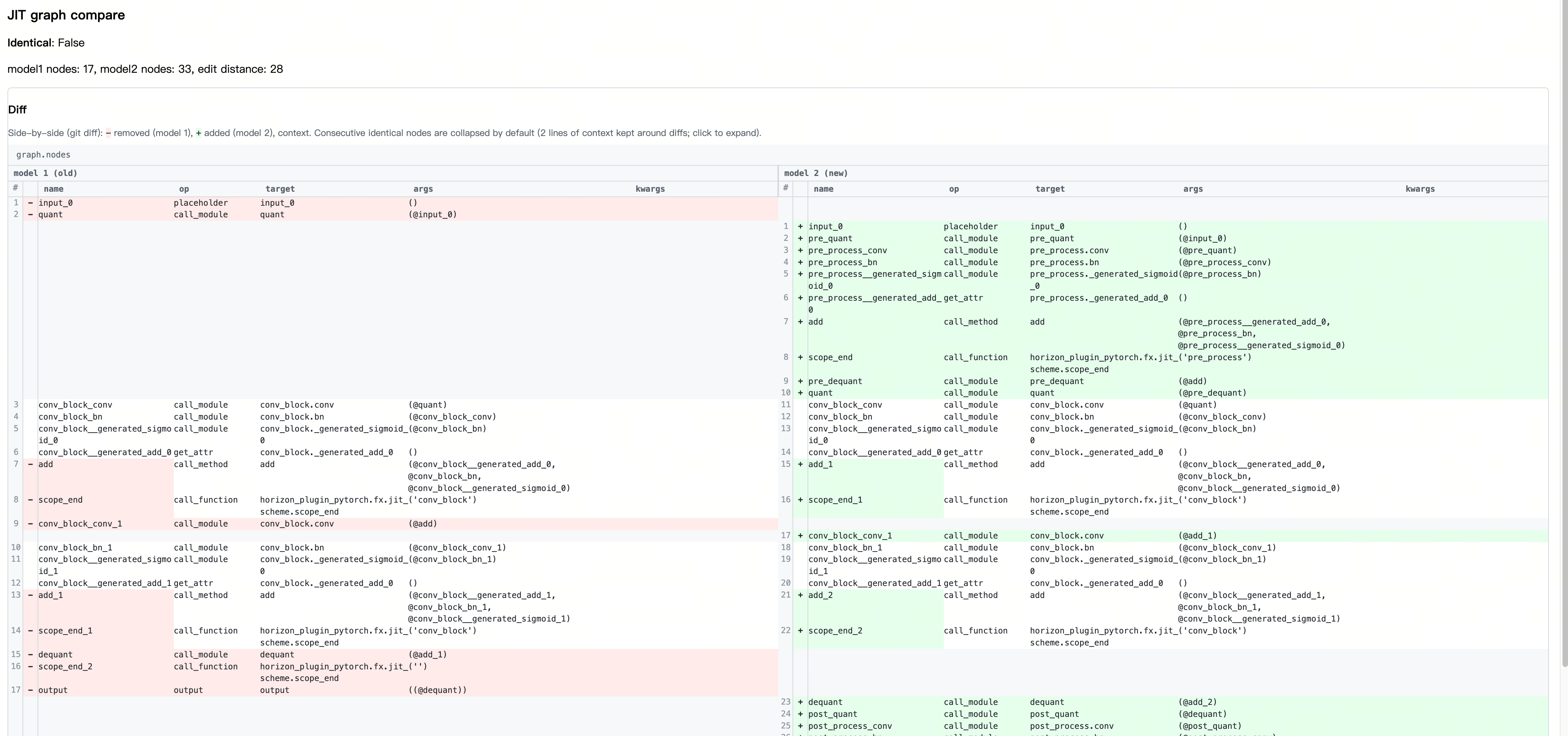
• Left side: Reference graph (model 1 / old).
• Right side: Current Prepare graph (model 2 / new).
• - red background: Nodes that exist only in the reference graph.
• + green background: Nodes that exist only in the current graph.
• Blank / white background: Aligned nodes with identical fields.
• Consecutive identical rows: Collapsed by default; click the blue summary bar to expand.

The run log also outputs the report path, for example: JIT graph compare HTML written to .../graph_compare.html.

#Risks That Need Special Attention

#Dynamic Code Blocks, Deploy Branches, and Changes in Loop Counts

The following coding patterns are the most likely to make the captured graph differ from expectations:

1. Training and deployment use different branches, such as if self.training or if deploy.

2. There are dynamic paths in forward that depend on condition checks.

3. The loop count differs across scenarios.

4. Some modules are defined in init, but are not actually called in the current Prepare forward path.

In these cases, the most important thing is not to guess which step went wrong first, but to use fx_graph.txt first to confirm what graph the tool is actually processing.

If a dynamic code block involves operator replacement or operator fusion, it must be explicitly marked with something like Tracer.dynamic_block. Otherwise, quantization information may become inconsistent, fusion results may become abnormal, or even the forward path may fail.

A typical usage looks like this:

from horizon_plugin_pytorch.fx.jit_scheme import Tracer

for _ in range(n):
    for _ in range(m):
        with Tracer.dynamic_block(self, "ConvBnAdd"):
            x = self.conv(x)
            x = self.bn(x)
            x = x + y

What really needs to be marked here is the code block inside the dynamic loop that involves operator replacement or operator fusion, rather than the for loop itself.

#Function Operator Replacement and Scope

Function operator replacement relies on the computation graph. Multiple calls to the same line of code in the graph are expanded into multiple nodes, so they may also be replaced by multiple Modules. If the model contains code blocks whose call counts differ between training and inference, scale misalignment may occur and further affect model accuracy.

To address this issue, the original implementation introduces the concept of Scope. Within the same Scope, the same func code call is replaced by the same shared Module. There are two common ways to define Scope:

1. The forward method of a Module type.

2. A code block marked with dynamic_block.

In addition, Prepare uses hooks to complete part of the wrapping and unwrapping of Wrappers. Therefore, after Prepare is completed, please do not modify any hooks in the model, otherwise the replacement may fail and cause errors or accuracy issues.

#Try to Isolate Deployment Logic

When using graph-based Prepare, it is best to ensure that the forward path entering Prepare contains only deployment logic. If training branches, loss computation, or other non-deployment logic are mixed into it directly, it becomes much easier for the captured graph to differ from the final deployment logic.

The following is a more robust example:

# Only apply prepare to deployment logic
def forward_infer(self, input, gt):
    conv_out = self.conv(input)
    return self.sigmoid(conv_out), conv_out

# Keep non-deployment logic outside
def forward(self, input, gt):
    sig_out, conv_out = self.forward_infer(input, gt)
    if self.training:
        return self.loss(conv_out, gt)
    return sig_out

If the code cannot temporarily isolate clean deployment logic because of readability or maintainability concerns, it is recommended to at least perform the following two additional checks:

1. Check whether there are missing key and unexpected key when loading ckpt. If quantization parameters are missing or extra, it often means the forward path of this Prepare run is not aligned with the path used when saving the ckpt.

2. Compare whether the fx_graph.txt generated by multiple Prepare runs is consistent. If the generated graph structure itself is inconsistent across runs, it usually means there are unstable factors in the forward path, and you should first judge whether that is expected.

#Exception Handling

If you have already found abnormalities in the Prepare stage, you can usually continue in the following directions:

• If you still cannot understand model_check_result.txt, fx_graph.txt, or the dtype inspection results, it is recommended to read Debug Artifacts Interpretation first.

• If you suspect that the graph structure changes after Prepare, the exported graph is inconsistent, or the training and deployment paths themselves are inconsistent, it is recommended to continue reading Deployment Consistency Analysis.

• If the issue looks more like the template configuration, dtype configuration, or high-precision output strategy itself is not as expected, it is recommended to return to Build QConfig and continue adjusting it.

• If the inspection results in the Prepare stage are basically normal, the next step is usually to continue to Calibration.