#Precision Tuning Guide

When results after prepare, Calibration, PyTorch QAT, or mixed precision configuration still do not meet expectations, you can continue troubleshooting and tuning in this section.

This section focuses on troubleshooting and tuning for PyTorch models during prepare, Calibration, PyTorch QAT, and mixed precision tuning.

This section mainly helps answer two questions:

• If the quantization pipeline has already been verified to run correctly but accuracy is still insufficient, where should the troubleshooting be narrowed down first?

• If a problematic stage or a set of problematic modules has already been identified, how should mixed precision configuration, debug artifacts, and accuracy analysis tools be used to narrow the issue down further?

If you have not yet confirmed that the pipeline itself is correct, it is recommended to return first to PyTorch Model Quantization Basic Workflow, Build Floating-point Model, Build QConfig, and Deployment Consistency Analysis to rule out workflow and configuration issues first.

Different methods are better at solving different kinds of problems. It is recommended to judge them in the following order:

1. If accuracy after Calibration is below expectation and routine checks still cannot narrow the issue quickly, start with step-by-step quantization to identify which stage or module the problem is mainly concentrated in.

2. If a specific stage or key layer has already been identified, or if per-layer comparison shows that the error becomes obviously larger at some layers, continue with histogram analysis and per-layer statistics to judge whether the issue is truncation, saturation, long-tail distribution, unreasonable scale, or something similar.

3. If you have already confirmed that mixed precision is needed to further improve accuracy, and you need to decide which operators are worth raising to int16 / fp16, continue with sensitivity analysis results to configure high-precision operators.

4. If the issue is still at the level of model structure, shared modules, fusion result, or qconfig correctness, finish model structure and quantization configuration checks first before moving on to later tuning.

#Background

#Quantization Error

The standard symmetric quantization formula is $quantized = clamp(round(\frac{float}{scale}), qmin, qmax)$. Errors mainly come from the following places:

1. Rounding error introduced by round. For example, when int8 quantization is used and scale is 0.0078, the fixed-point value of floating-point value 0.0157 is round(0.0157 / 0.0078) = round(2.0128) = 2, and the fixed-point value of floating-point value 0.0185 is round(0.0185 / 0.0078) = round(2.3718) = 2. Both values produce rounding error, and because of rounding, they also map to the same fixed-point value.

2. Truncation error introduced by clamp. When qmax * scale cannot cover the value range that needs to be quantized, the truncation error may become large. For example, when int8 quantization is used and scale is 0.0078, then qmax * scale = 127 * 0.0078 = 0.9906, and values greater than 0.9906 will be truncated to 127.

Quantization always introduces error, but the impact of that error on final model accuracy differs for several reasons:

1. Some outliers may have large truncation error but almost no effect on final model accuracy.

2. Different operators have different sensitivity to error. For example, operators such as sigmoid and softmax usually tolerate input error better in certain domains, while operators such as topk and sort are very sensitive to error.

3. A model itself has some robustness and generalization ability, and small errors may even behave like a form of regularization during training.

#Reducing Quantization Error

1. For rounding error, a smaller scale can be used so that each fixed-point value corresponds to a smaller floating-point interval. Since reducing scale directly will also increase truncation risk, the common way is to use a higher precision dtype, for example replacing int8 with int16. Because the fixed-point range becomes larger, scale becomes smaller as well.

2. For truncation error, a larger scale can be used. In practice, scale is generally obtained by quantization tools through statistics. If scale is too small, common reasons are that calibration data is not comprehensive enough, or the calibration method is not suitable, which makes the collected scale unreasonable. For example, if the theoretical input range is [-1, 1] but no samples near 1 or -1 are observed during calibration or QAT, or such samples appear too rarely, the estimated scale may be too small. In that case, more such data should be added or a fixed scale should be set manually according to the expected numeric range. When truncation is not too severe, calibration parameters can also be adjusted, and different calibration methods or hyperparameters can be tried to mitigate truncation error.

#Quantization Accuracy Tuning

Quantization accuracy tuning includes two parts:

1. Model structure and quantization configuration checks. The main purpose of these checks is to avoid non-tuning issues from affecting quantized accuracy, such as incorrect qconfig settings or quantization-unfriendly shared modules.

2. Mixed precision tuning. First use a model dominated by high-precision operators to quickly iterate to a model that meets the accuracy target, so that the accuracy upper bound and performance lower bound can be obtained. Then use accuracy tuning tools to analyze and adjust the quantization configuration and finally produce a quantized model that balances accuracy and performance.

#Common Troubleshooting Methods

#Step-by-step Quantization

Step-by-step quantization is meant for narrowing down the scope first, rather than deciding the final configuration directly.

The basic idea is to introduce quantization gradually by model stage, submodule, or local fragment, and observe where the error starts to increase significantly. If accuracy clearly recovers after fake quantization is disabled for a certain part, the issue is usually concentrated there.

This method is especially suitable in the following cases:

• Accuracy after Calibration is below expectation, and it is still hard to tell whether the issue looks more like a structure problem, an input distribution problem, or a local quantization configuration problem.

• The model is large, and directly examining full per-layer results is too expensive, so you want to narrow the scope first by larger blocks such as backbone, neck, or head.

• Routine parameter adjustments have already been tried, but it is still unclear where the error starts to grow.

If the earlier judgment is still not clear enough, you can go a step further and directly disable fake quantization for certain parts of the model, then compare model accuracy with fake quantization enabled and disabled. If accuracy clearly recovers after one segment is disabled, the issue is usually in that segment. For floating-point computation, fake cast can also be turned on and off for comparison.

The following is an example that keeps head out of quantization:

from horizon_plugin_pytorch.utils.quant_switch import GlobalFakeQuantSwitch
from horizon_plugin_pytorch.quantization.fake_cast import FakeCast

# Example: do not quantize the head
class Model(nn.Module):
    def _init_(...):
    def forward(self, x):
        x = self.quant(x)
        x = self.backbone(x)
        x = self.neck(x)
        GlobalFakeQuantSwitch.disable()  # Disable fake quantization
        FakeCast.disable()  # Disable fake cast
        x = self.head(x)
        GlobalFakeQuantSwitch.enable()  # Enable fake quantization
        FakeCast.enable()  # Enable fake cast
        return self.dequant(x)

#Histogram Analysis

Histogram analysis is suitable when some layers already look suspicious and you want to understand why they are suspicious.

It is usually used together with the input, output, or activation distribution of key layers to further judge whether the error looks more like truncation, saturation, long-tail distribution, unreasonable scale, or abnormal numeric range.

When per-layer comparison has already shown that the error becomes obviously larger from a certain layer onward, do not stop at simply concluding that the layer has large error. It is better to continue with distribution information and determine whether the real issue is that the statistical range is too small, the quantization resolution is insufficient, or the model data itself contains abnormal ranges.

If the current issue looks more like inaccurate activation statistics, or if you already suspect that the default scale search method is not suitable for the current model, start with HistogramObserver. It collects more complete distribution information over the whole calibration set and then computes scale with a search strategy. Compared with methods that record only min and max and then update them with moving average, the histogram method is usually more stable and is often a better default starting point for activation calibration.

In practical troubleshooting, histogram analysis usually focuses on the following signals:

• The main body of the distribution is concentrated, but a small number of outliers stretch the range very far. In that case, scale can be dominated by a few abnormal values, and the quantization resolution for the normal range becomes insufficient.

• The distribution is clearly flattened near the boundary, or many samples pile up around upper and lower limits. This usually means the current scale is too small and truncation or saturation has already appeared.

• The distribution does not show obvious truncation, but the effective numeric range is still very wide and the resolution in important intervals is still insufficient. This usually looks more like the current quantization dtype is not enough, or that some local operators need to be raised to higher precision.

• The same module is called multiple times and the distributions differ greatly across calls. Even if each single observation looks normal, sharing one set of quantization parameters may still keep amplifying the error.

If the main issue lies in the activation scale search method rather than the data itself or the model structure, the histogram method has another practical advantage. Statistics collection and scale calculation can be handled separately. In other words, after one calibration run is complete, you can directly use HistogramObserver.reset_scale to switch search methods and recompute scale without rerunning the full calibration dataset.

A common usage pattern is to finish activation statistics with HistogramObserver during Calibration, then switch the search method through reset_scale according to evaluation results and observe whether the key layers or overall accuracy improve.

import torch

from horizon_plugin_pytorch.quantization import (
    FakeQuantState,
    QconfigSetter,
    get_qconfig,
    prepare,
    qint8,
    qint16,
    set_fake_quantize,
)
from horizon_plugin_pytorch.quantization.observer_v2 import HistogramObserver
from horizon_plugin_pytorch.quantization.qconfig_setter import (
    ConvDtypeTemplate,
    MatmulDtypeTemplate,
    ModuleNameTemplate,
)

# 1. Build the calibration qconfig with HistogramObserver
qconfig_setter = QconfigSetter(
    reference_qconfig=get_qconfig(observer=HistogramObserver),
    templates=[
        ModuleNameTemplate({"": qint8}),
        ConvDtypeTemplate(input_dtype=qint8, weight_dtype=qint8),
        MatmulDtypeTemplate(input_dtypes=qint8),
    ],
)

calib_model = prepare(
    model,
    example_inputs=example_inputs,
    qconfig_setter=qconfig_setter,
)
calib_model.eval()

# 2. Run one pass of calibration data to finish histogram collection
set_fake_quantize(calib_model, FakeQuantState.CALIBRATION)
with torch.no_grad():
    for example_inputs in calib_loader:
        calib_model(example_inputs)

# 3. Switch the scale search method for qint8 activations without recalibrating
HistogramObserver.reset_scale(
    calib_model,
    method="percentile",
    method_kwargs={"percentile": 0.999999},
    dtype=qint8,
)

# 4. If some int16 nodes need to preserve a more complete range, recompute qint16 scale separately
HistogramObserver.reset_scale(
    calib_model,
    method="percentile",
    method_kwargs={"percentile": 1.0},
    dtype=qint16,
)

# 5. Save the state_dict again after reset_scale, then evaluate or export
torch.save(calib_model.state_dict(), "calib_model.pth")

If you have already narrowed the issue down to a specific branch or module, you can also use prefix to recompute scale only within the specified scope. Whether prefix is used or not, it is still recommended to finish reset_scale before evaluation or export, and then save the state_dict again. If you later decide to raise some nodes to higher precision through reset_dtype, it is also recommended to recompute the corresponding scale after the dtype change before continuing evaluation or export.

The common search methods can be understood like this first:

The smaller percentile is, the more aggressive the truncation becomes. If the current error mainly comes from a small number of extreme values stretching the range too far, moderately lowering percentile often helps reserve more quantization resolution for the main distribution. On the other hand, if some int16 nodes are expected to preserve the full range as much as possible, percentile can also be adjusted to 1.0 so that the result is closer to minmax.

This kind of analysis is most suitable during the Calibration stage. If calibration has already been completed once, keep the calibration dataset fixed and adjust only the search method and parameters in reset_scale, then compare the result changes. That usually helps determine more quickly whether the issue comes from the scale search strategy, or from model structure, data distribution, or quantization dtype itself.

#Sensitivity Analysis

Sensitivity analysis is suitable when deciding which operators are worth raising to higher precision.

Its main purpose is to identify operators that have a larger impact on final model output according to quantization sensitivity results, and to provide evidence for deciding whether related operators should be raised to int16 / fp16.

Once the initial localization work is done and you are about to enter mixed precision tuning, sensitivity analysis is usually the key basis for deciding the proportion and placement of high-precision operators.

#Model Structure and Quantization Configuration Checks

After the model has completed prepare, it is recommended to first check for incorrect quantization configuration and for model structures that are unfriendly to quantization. This can be done with the check_qat_model interface in the debug tools. For usage details, refer to Accuracy Tuning Tool Guide.

#Operator Fusion

Check whether there are modules in the model that can be fused but were not actually fused. During BPU deployment, operators such as conv, bn, add, and relu are fused. In a QAT model, these operators are replaced by one module to avoid inserting fake quantization nodes in the middle. If these operators are not fused, extra quantization nodes will appear in the middle and may have a slight impact on both accuracy and performance. The following example shows that conv and relu were not fused.

Fusable modules are listed below:
name    type
------  -----------------------------------------------------
conv    <class 'horizon_plugin_pytorch.nn.qat.conv2d.Conv2d'>
relu    <class 'horizon_plugin_pytorch.nn.qat.relu.ReLU'>

Under different methods of prepare, the reasons and fixes for fusion errors may differ:

1. PrepareMethod.JIT and PrepareMethod.JIT_STRIP:

   a. If operator fusion exists inside dynamic code blocks, those blocks need to be marked with dynamic_block.

   b. If the parts with changing call counts execute only once during tracing, example_inputs should be chosen so that those parts execute multiple times.

2. PrepareMethod.EAGER: if fuse was not performed or fuse_modules was written incorrectly, the handwritten fuse logic needs to be checked and fixed.

#Shared Modules

Because horizon_plugin_pytorch inserts quantization nodes through module replacement, only one set of quantization information can be collected for each module. When one module object is called multiple times and the output distributions across those calls differ greatly, using one shared set of quantization parameters may produce large error, and the shared module should be split. If the distributions across those calls do not differ much, splitting is unnecessary. This section first explains what shared modules mean here, and later during per-layer comparison you can use this result to decide whether the shared module needs to be split.

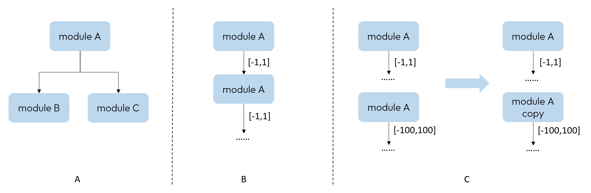
The similarities and differences between three common understandings of sharing and the sharing discussed here are as follows:

A. One module is followed by multiple modules, and module A is considered shared. However, module A is actually called only once here, so there is no output distribution difference. It does not affect quantized accuracy, and it also does not appear in the call-count check.

B. One module is called repeatedly, but the output distributions across calls are similar. This can be seen in the call-count check, but the impact on quantized accuracy is small, so no change is needed.

C. One module is called repeatedly and the output distributions across calls differ greatly. This can be seen in the call-count check and usually has a large impact on quantized accuracy, so the module needs to be manually copied and split.

In model_check_result.txt, you can inspect the call count of each module. Normally each op is called only once. 0 means it was not called, and a value greater than 1 means it was called multiple times. In the example below, conv is a shared module.

Each module called times:
name       called times
-------  --------------
conv                  2
quant                 1
dequant               1

# Corresponding code
# def forward(self, x):
#     x = self.quant(x)
#     x = self.conv(x)
#     x = self.conv(x)
#     x = self.dequant(x)
#     return x

#QConfig Configuration Errors

Incorrect qconfig usage may cause the model to be quantized in a way different from what was intended, which can then lead to accuracy loss. For example, template settings and qconfig attribute settings may be mixed together. Here the main check is whether the input and output of each operator in model_check_result.txt match expectations:

1. Whether dtype matches the configuration.

2. Whether high-precision output is enabled.

Each layer out qconfig:
+---------------+-----------------------------------------------------------+---------------+---------------+----------------+-----------------------------+
| Module Name   | Module Type                                               | Input dtype   | out dtype     | ch_axis        | observer                    |
|---------------+-----------------------------------------------------------+---------------+---------------+----------------+-----------------------------|
| quant         | <class 'horizon_plugin_pytorch.nn.qat.stubs.QuantStub'>   | torch.float32 | qint8         | -1             | MovingAverageMinMaxObserver |
| conv          | <class 'horizon_plugin_pytorch.nn.qat.conv2d.Conv2d'>     | qint8         | qint8         | -1             | MovingAverageMinMaxObserver |
| relu          | <class 'horizon_plugin_pytorch.nn.qat.relu.ReLU'>         | qint8         | qint8         | qconfig = None |                             |
| dequant       | <class 'horizon_plugin_pytorch.nn.qat.stubs.DeQuantStub'> | qint8         | torch.float32 | qconfig = None |                             |
+---------------+-----------------------------------------------------------+---------------+---------------+----------------+-----------------------------+
# The result here shows all modules are quantized as int8. If you configured int16, the configuration did not take effect and qconfig usage needs to be checked.
Weight qconfig:
+---------------+-------------------------------------------------------+----------------+-----------+---------------------------------------+
| Module Name   | Module Type                                           | weight dtype   |   ch_axis | observer                              |
|---------------+-------------------------------------------------------+----------------+-----------+---------------------------------------|
| conv          | <class 'horizon_plugin_pytorch.nn.qat.conv2d.Conv2d'> | qint8          |         0 | MovingAveragePerChannelMinMaxObserver |
+---------------+-------------------------------------------------------+----------------+-----------+---------------------------------------+

In addition, model_check_result.txt may also contain abnormal qconfig warnings, such as abnormal qconfig prompts. These items are qconfig settings that the tool suggests should be checked again. They need to be judged together with the actual scenario and are not necessarily wrong. For example, in the fixed scale prompt shown below, you need to check whether the fixed scale setting for that layer is really expected.

Please check if these OPs qconfigs are expected..
+-----------------+----------------------------------------------------------------------------+------------------------------------------------------------------+
| Module Name     | Module Type                                                                | Msg                                                              |
|-----------------+----------------------------------------------------------------------------+------------------------------------------------------------------|
| sub[sub]        | <class 'horizon_plugin_pytorch.nn.qat.functional_modules.FloatFunctional'> | Fixed scale 3.0517578125e-05                                     |
+-----------------+----------------------------------------------------------------------------+------------------------------------------------------------------+

#Common Mixed Precision Tuning Workflow

Whether you are on J6E/M or J6P, mixed precision tuning usually does not begin by deciding the final high-precision ratio right away. A more common order is to finish basic tuning and advanced tuning first, and then use accuracy tuning tools to gradually decide the scope and proportion of high-precision operators.

#Basic Tuning Methods

Basic tuning methods are more suitable for quick iteration. Whether you are doing full int16 tuning or full int8 tuning, models at this stage are usually only intermediate states for quick validation, so it is generally better to start with basic tuning methods. Only when mixed precision tuning needs to further reduce the proportion of high-precision operators is it recommended to move on to more complex advanced tuning methods. That introduces more trial and error and more iteration cost, but it also usually gives a better chance of balancing both accuracy and performance.

#Calibration

1. Adjust calibration steps. More calibration data is generally better, but because of diminishing returns, the gain in accuracy becomes very limited after the data amount reaches a certain level. If the training set is small, it can all be used for calibration. If the training set is large, choose a suitable subset according to calibration cost, and it is recommended to run at least 10 - 100 calibration steps.

2. Adjust batch size. In general, batch size should be as large as possible. If the data is noisy or the model has many outliers, it can be reduced appropriately.

3. Use inference-time preprocessing together with training data for calibration. Calibration data should be close to the real distribution. Augmentations such as flipping can be used, while augmentations such as rotation and mosaic that change the real distribution should not be used.

#QAT

1. Adjust learning rate.

   a. Initial learning rate: remove warmup, remove learning rate decay strategy, use different fixed learning rates such as 1e-3, 1e-4, and so on to finetune for a small number of steps, observe evaluation metrics, and choose the best one as the initial learning rate. If different modules used different learning rates in float training, those combinations should also be tried here.

   b. Scheduler: align the learning rate decay strategy with the float training setup, but make sure there is no warmup-like strategy. For example, if float training uses cosine annealing, QAT should also use cosine annealing.

2. Try both strategies of fixing and updating input and output scale. In general, when calibration model accuracy is already good, fixing input and output scale for QAT training often gives better results. When calibration accuracy is poor, it is usually not suitable to fix it. There is no single metric that decides this in advance, so both strategies usually need to be tried.

3. The number of training steps is generally no more than 20% of float training, and can be adjusted according to training loss and evaluation result.

Points that need special attention:

1. Except for the items above that need adjustment, the rest of the QAT training configuration should align with float training.

2. If float training uses techniques such as freeze bn, then QAT training needs to set qat mode to withbn.

from horizon_plugin_pytorch.qat_mode import QATMode, set_qat_mode
set_qat_mode(QATMode.WithBN)

from horizon_plugin_pytorch.quantization import set_fake_quantize, FakeQuantState
# This also applies when troubleshooting calibration accuracy issues
set_fake_quantize(model, FakeQuantState._FLOAT)

#Advanced Tuning Methods

Advanced tuning methods usually require more time and repeated trial and error, so they are more suitable when the accuracy target is high and the basic methods still cannot satisfy the requirement. Common approaches include the following.

#Set Fixed Scale

For some parts of the model, it is difficult to obtain the optimal quantization scale only through statistics. A common case where fixed scale is needed is when the output value range of an operator is already known.

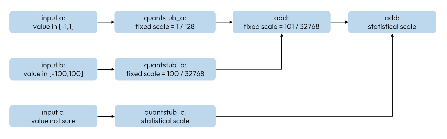
For example, if the input data is speed in km / h and the value range is [0, 200], then for quantstub, the output range is fixed and the scale should be set to 200 / quantized numeric range. The reason is that quantization scale is normally obtained through statistics, and with ordinary calibration data it is hard to guarantee that every sample reaches boundary cases. Statistical methods often use moving averages to suppress outliers, which causes the obtained quantization range to be smaller than the real range. In the speed example above, if fixed scale is not set, the estimated maximum speed may become close to the average speed of most vehicles, which makes all samples above that speed suffer obvious accuracy loss at input time. It may be hard to identify all places that need fixed scale at this stage, but such problems are usually easy to discover during the per-layer comparison step of accuracy debugging.

In the figure below, input a and b have known ranges, while input c does not. Except for quantstub_c and the later add, all the other operators need fixed scale.

#Calibration

Try different calibration methods. For activation statistics, it is recommended to prioritize HistogramObserver. The plugin supports multiple histogram-based scale search methods. Besides the default mse, you can also try different percentile configurations. For example, if you suspect the accuracy drop is caused by truncation, try different percentile parameters. After one calibration run is completed, scale can also be recomputed through HistogramObserver.reset_scale without recalibrating. For interface usage, refer to Calibration Guide.

#QAT

1. Adjust weight decay. Weight decay affects the numeric range of weights in the model. A smaller numeric range is usually more quantization-friendly. Sometimes adjusting weight decay only in the QAT stage is still not enough, and weight decay in the float training stage also needs to be adjusted.

2. Adjust data augmentation. Quantized models generally have weaker learning ability than float models. Overly strong augmentation may affect convergence of QAT models, so augmentation usually needs to be weakened appropriately.

#Accuracy Tuning Tool Workflow

Once basic tuning and advanced tuning have been tried, the next step is usually to use accuracy tuning tools to decide the scope and proportion of high-precision operators. This workflow is basically shared across J6E/M and J6P.

The core of this debug stage is to compare the floating-point model with the calibration model. It is generally not recommended to compare the floating-point model directly with the QAT model, because after Quantized Awareness Training the two models are no longer in a state suitable for direct comparison. It is recommended to read Accuracy Tuning Tool Guide first for related background, then provide a dataset to locate badcases with large loss in the calibration model, and continue from those badcases with per-layer comparison and quantization sensitivity analysis.

#Find Badcases

Most of the later accuracy debug work revolves around badcases. You need to provide a sample set where quantized accuracy is poor. The tool will iterate through the sample set and compare the output error of the floating-point model and the calibration model on each sample. In most cases, no extra error metric function is needed.

Use the auto_find_bad_case interface in the debug tool to find badcases as shown below:

from horizon_plugin_profiler.model_profilerv2 import QuantAnalysis

# 1. Initialize the quantization analysis object
qa = QuantAnalysis(float_net, calibration_model, "fake_quant")

# 2. Find badcases. If the dataset is large, num_steps can be specified to search only part of the data
qa.auto_find_bad_case(dataloader)

After badcase search is finished, inspect the result file. For every model output and every error metric, the debug tool picks one worst sample. In the example below, the model has three outputs. The first table shows the worst sample index for each output under each metric. The second table shows the corresponding error values. The third table shows the badcase index of the worst output under the current metric.

The bad case input index of each output:
Name/Index    COSINE    L1    ATOL
------------  --------  ----  ------
0-0           4         1     1
0-1           14        1     1
0-2           12        9     9

The metric results of each badcase:
Name/Index    COSINE    L1         ATOL
------------  --------  ---------  ---------
0-0           0.969289  0.996721   11.9335
0-1           0.974127  0.0404785  12.6742
0-2           0.450689  1.08771    20.821809

The bad case input index of the worst output:
metric    dataloader index
--------  ------------------
COSINE    11
L1        17
ATOL      0

#Per-layer Comparison

Per-layer comparison runs the floating-point model and the calibration model on the specified badcase, then compares the output of every layer and computes corresponding statistics and error values. This can be done with the compare_per_layer interface in the debug tool. If the accuracy loss is not yet obvious, or the problem scope is still too broad, this step can be skipped first and revisited later together with sensitivity results.

from horizon_plugin_profiler.model_profilerv2 import QuantAnalysis

# 1. Initialize the quantization analysis object
qa = QuantAnalysis(float_net, calibration_model, "fake_quant")

# 2. Find badcases. If the dataset is large, num_steps can be specified to search only part of the data
qa.auto_find_bad_case(dataloader)

# 3. Run the models on the badcase and collect per-layer information
qa.run()

# 4. Compare the collected per-layer information
qa.compare_per_layer()

The per-layer comparison result can be examined in the generated text file. In that file, read from top to bottom to find the operator where the error starts to be amplified.

+------+----------------------------------------+-----------------------------------------------------------------------------+-----------------------------------------------------------+---------------------------------------+---------------+-----------+------------+-----------------+--------------+------------+--------------+---------------+-------------------+--------------------+--------------------+--------------------+--------------------+--------------------+--------------------+--------------------+--------------------+-----------------+-------------------+
|      | mod_name                               | base_op_type                                                                | analy_op_type                                             | shape                                 | quant_dtype   |    qscale |     Cosine |             MSE |           L1 |         KL |         SQNR |          Atol |              Rtol |     base_model_min |    analy_model_min |     base_model_max |    analy_model_max |    base_model_mean |   analy_model_mean |     base_model_var |    analy_model_var |   max_atol_diff |   max_qscale_diff |
|------+----------------------------------------+-----------------------------------------------------------------------------+-----------------------------------------------------------+---------------------------------------+---------------+-----------+------------+-----------------+--------------+------------+--------------+---------------+-------------------+--------------------+--------------------+--------------------+--------------------+--------------------+--------------------+--------------------+--------------------+-----------------+-------------------|
|    0 | backbone.quant                         | horizon_plugin_pytorch.quantization.stubs.QuantStub                         | horizon_plugin_pytorch.nn.qat.stubs.QuantStub             | torch.Size([4, 3, 512, 960])          | qint16        | 0.0078125 |  0.9999999 |       0.0000000 |    0.0000000 |  0.0000000 |  inf         |     0.0000000 |         0.0000000 |         -1.0000000 |         -1.0000000 |          0.9843750 |          0.9843750 |         -0.1114422 |         -0.1114422 |          0.1048462 |          0.1048462 |       0.0000000 |         0.0000000 |
|    1 | backbone.mod1.0                        | torch.nn.modules.conv.Conv2d                                                | horizon_plugin_pytorch.nn.qat.conv_bn2d.ConvBN2d          | torch.Size([4, 32, 256, 480])         | qint16        | 0.0003464 |  0.4019512 |       0.4977255 |    0.4296696 |  0.0115053 |   -0.3768753 |    14.2325277 |   5343133.5000000 |         -5.9793143 |        -15.0439596 |          8.7436047 |         17.3419971 |          0.1503869 |          0.0484397 |          0.4336909 |          0.3707855 |      14.2325277 |     41088.2696619 |
|    2 | backbone.mod1.1                        | torch.nn.modules.batchnorm.BatchNorm2d                                      | torch.nn.modules.linear.Identity                          | torch.Size([4, 32, 256, 480])         | qint16        | 0.0003464 |  0.9999998 |       0.0000000 |    0.0000000 |  0.0000000 |  inf         |     0.0000000 |         0.0000000 |        -15.0439596 |        -15.0439596 |         17.3419971 |         17.3419971 |          0.0484397 |          0.0484397 |          0.3707855 |          0.3707855 |       0.0000000 |         0.0000000 |
|    3 | backbone.mod2.0.head_layer.conv.0.0    | torch.nn.modules.conv.Conv2d                                                | horizon_plugin_pytorch.nn.qat.conv_bn2d.ConvBNReLU2d      | torch.Size([4, 64, 256, 480])         | qint16        | 0.0004594 |  0.5790146 |      49.3001938 |    4.0790396 |  0.0415040 |    0.3848250 |   164.3788757 |   4046676.7500000 |       -164.3788757 |          0.0000000 |        140.9307404 |         25.1951389 |         -0.5375993 |          0.2460073 |         53.5661125 |          0.2699530 |     164.3788757 |    357789.3997821 |
|    4 | backbone.mod2.0.head_layer.conv.0.1    | torch.nn.modules.batchnorm.BatchNorm2d                                      | torch.nn.modules.linear.Identity                          | torch.Size([4, 64, 256, 480])         | qint16        | 0.0004594 |  0.7092103 |       0.3265578 |    0.2332140 |  0.0003642 |    3.0239849 |    17.1071243 |         1.0000000 |        -17.1071243 |          0.0000000 |         25.1951389 |         25.1951389 |          0.0127933 |          0.2460073 |          0.6568668 |          0.2699530 |      17.1071243 |     37235.6102222 |
|    5 | backbone.mod2.0.head_layer.conv.0.2    | torch.nn.modules.activation.ReLU                                            | torch.nn.modules.linear.Identity                          | torch.Size([4, 64, 256, 480])         | qint16        | 0.0004594 |  1.0000001 |       0.0000000 |    0.0000000 |  0.0000000 |  inf         |     0.0000000 |         0.0000000 |          0.0000000 |          0.0000000 |         25.1951389 |         25.1951389 |          0.2460073 |          0.2460073 |          0.2699530 |          0.2699530 |       0.0000000 |         0.0000000 |
|    6 | backbone.mod2.0.head_layer.short_add   | horizon_plugin_pytorch.nn.quantized.functional_modules.FloatFunctional.add  | horizon_plugin_pytorch.nn.qat.conv_bn2d.ConvBNAddReLU2d   | torch.Size([4, 32, 256, 480])         | qint16        | 0.0004441 |  0.5653002 |       1.6375992 |    0.4214573 |  0.0008538 |    1.6659310 |    39.9804993 |         1.0000000 |        -39.9804993 |          0.0000000 |         19.6796150 |         19.6796150 |          0.0330326 |          0.4544899 |          2.4056008 |          0.5625318 |      39.9804993 |     90017.7454165 |
|    7 | backbone.mod2.0.head_layer.relu        | torch.nn.modules.activation.ReLU                                            | torch.nn.modules.linear.Identity                          | torch.Size([4, 32, 256, 480])         | qint16        | 0.0004441 |  1.0000000 |       0.0000000 |    0.0000000 |  0.0000000 |  inf         |     0.0000000 |         0.0000000 |          0.0000000 |          0.0000000 |         19.6796150 |         19.6796150 |          0.4544899 |          0.4544899 |          0.5625318 |          0.5625318 |       0.0000000 |         0.0000000 |

#Compute Quantization Sensitivity

This step evaluates the effect of each quantization node on final accuracy and can be performed with the sensitivity interface in the debug tool. The basic idea is to use badcases as model input, enable each quantization node one by one, and then compare the error between the quantized model and the floating-point model. The error metric used here is the same as the metric used during badcase search.

from horizon_plugin_profiler.model_profilerv2 import QuantAnalysis

# 1. Initialize the quantization analysis object
qa = QuantAnalysis(float_net, calibration_model, "fake_quant")

# 2. Find badcases. If the dataset is large, num_steps can be specified to search only part of the data
qa.auto_find_bad_case(dataloader)

# 3. Run the models on the badcase and collect per-layer information
qa.run()

# 4. Compare the collected per-layer information
qa.compare_per_layer()

# 5. Compute quantization sensitivity
qa.sensitivity()

In the quantization sensitivity result, operators ranked higher in sensitivity have a larger effect on final model accuracy and should be set to a higher precision dtype.

The sensitive_type column has two values, weight and activation, which indicate the case where only the weight quantization node or only the output quantization node of that operator is enabled.

op_name                                                                                                          sensitive_type    op_type                                                                           L1  quant_dtype
---------------------------------------------------------------------------------------------------------------  ----------------  --------------------------------------------------------------------------  --------  ------------
bev_stage2_e2e_dynamic_head.head.transformer.decoder.layers.5.cross_attn.quant                                   activation        <class 'horizon_plugin_pytorch.nn.qat.stubs.QuantStub'>                     1.59863   qint8
bev_stage2_e2e_dynamic_head.head.transformer.decoder.layers.5.norm3.var_mean.pre_mean                            activation        <class 'horizon_plugin_pytorch.nn.qat.functional_modules.FloatFunctional'>  1.52816   qint16
bev_stage2_e2e_dynamic_head.head.ref_pts_quant                                                                   activation        <class 'horizon_plugin_pytorch.nn.qat.stubs.QuantStub'>                     1.16427   qint8
bev_stage2_e2e_dynamic_head.head.fps_quant                                                                       activation        <class 'horizon_plugin_pytorch.nn.qat.stubs.QuantStub'>                     1.13563   qint8
bev_stage2_e2e_dynamic_head.head.transformer.decoder.mem_bank_layer.emb_fps_queue_add                            activation        <class 'horizon_plugin_pytorch.nn.qat.functional_modules.FloatFunctional'>  1.11997   qint8
bev_stage2_e2e_dynamic_head.head.transformer.decoder.mem_bank_layer.temporal_norm2.weight_mul                    activation        <class 'horizon_plugin_pytorch.nn.qat.functional_modules.FloatFunctional'>  1.09876   qint8

#J6E/M Mixed Precision Tuning

#Tuning Workflow

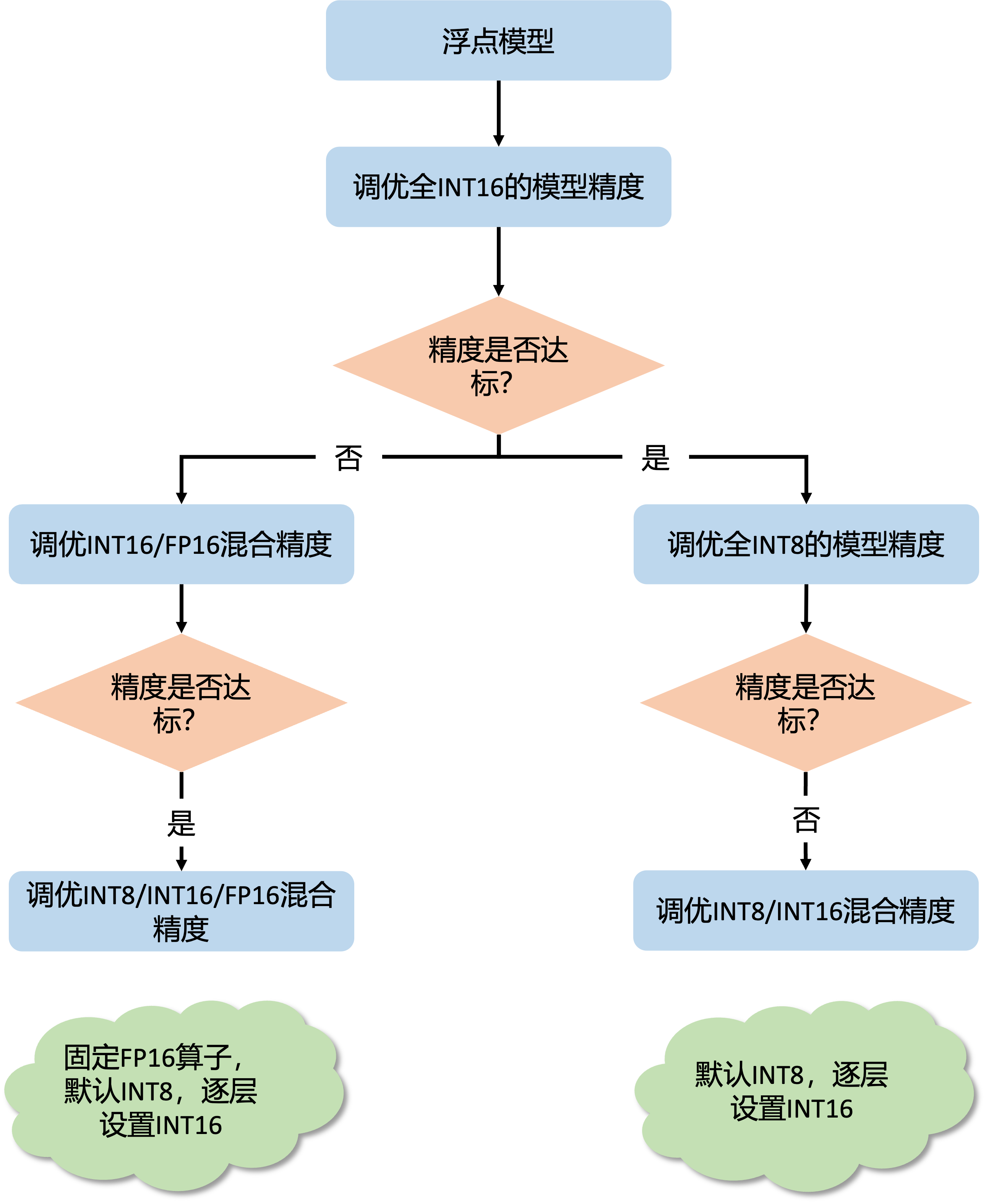
The full workflow usually starts from full int16. The main purpose of this step is to confirm the accuracy upper bound first, while also ruling out tool usage issues and quantization-unfriendly modules.

1. After full int16 is confirmed to meet the accuracy target, continue with full int8 tuning. If accuracy is still not sufficient, move on to int8 / int16 mixed precision tuning and gradually increase the proportion of int16 on top of the full int8 model. At this stage, you need to trade off accuracy and performance and find a quantization configuration with the best possible performance while still meeting the accuracy target.

2. If full int16 still does not meet the accuracy target, continue with int16 / fp16 mixed precision tuning. In the ideal case, int16 / fp16 mixed precision tuning can solve all accuracy problems. Then continue with int8 / int16 / fp16 mixed precision tuning, keep all fp16 operator settings fixed, and adjust the proportion of int16 operators using the same method as in item 1 for int8 / int16 mixed precision tuning.

Before entering the mixed precision configurations below, the platform-independent basic tuning methods, advanced tuning methods, and accuracy tuning tool workflow can be referenced in Basic Tuning Methods, Advanced Tuning Methods, and Accuracy Tuning Tool Workflow.

#INT8 / INT16 Mixed Precision Tuning and INT16 / FP16 Mixed Precision Tuning

The basic idea of mixed precision tuning is to start from a higher-precision configuration that is easier to meet the accuracy target, then gradually reduce the proportion of high-precision operators until a configuration that balances accuracy and performance is found. In int8 / int16 mixed precision tuning, the starting point is usually a full int8 model and int16 operators are gradually added. In int16 / fp16 mixed precision tuning, the starting point is usually a full int16 model and fp16 operators are gradually added.

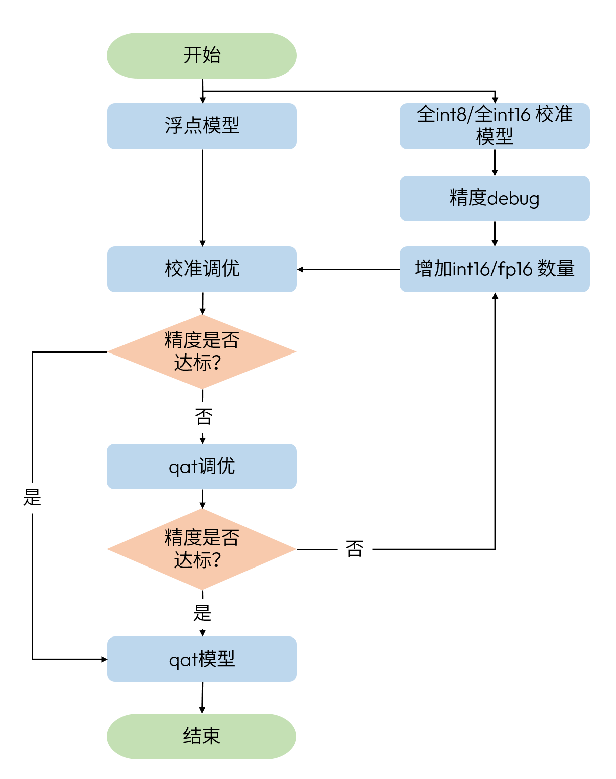
For the Calibration and QAT tuning shown in the figure above, refer to Basic Tuning Methods and Advanced Tuning Methods. As for how many int16 / fp16 high-precision operators should be added, that needs to be judged from the series of results produced by the accuracy debug tools.

How to find badcases, perform per-layer comparison, and compute quantization sensitivity in this stage can all be referenced directly in the earlier Accuracy Tuning Tool Workflow. The J6E/M section focuses more on how to turn those analysis results into int16 / fp16 configuration.

Sensitivity templates are needed here. For usage details, refer to Build QConfig. If the model has multiple outputs, a corresponding sensitivity table is generated for each output. You can select several sensitivity tables whose indicators differ significantly and configure sensitivity templates from them. The following example is for int8 / int16 mixed precision tuning, where the top 20% of int8 sensitivity results from two output sensitivity tables are set to int16. The total number of int16 operators is the union of the top 20% operators from the two tables. Then keep adjusting the int16 ratio until the minimum int16 ratio that satisfies the accuracy requirement is found.

qat_model = prepare(
    model,
    example_inputs=example_input,
    qconfig_setter=(
        sensitive_op_calibration_8bit_weight_16bit_act_qconfig_setter(table1, ratio=0.2),
        sensitive_op_calibration_8bit_weight_16bit_act_qconfig_setter(table2, ratio=0.2),
        default_calibration_qconfig_setter,
    )
)
qat_model = prepare(
    model,
    example_inputs=example_input,
    qconfig_setter=(
        sensitive_op_qat_8bit_weight_16bit_act_qconfig_setter(table1, ratio=0.2),
        sensitive_op_qat_8bit_weight_16bit_act_qconfig_setter(table2, ratio=0.2),
        default_qat_qconfig_setter,
    )
)

When tuning the amount of int16 for models with many outputs, the following experience can be used:

1. Adjust the ratio with binary search. Apply the same ratio to all sensitivity tables and tune it with binary search. After the accuracy target is met, reduce the high-precision ratio for individual sensitivity tables one by one, again with binary search.

2. Adjust according to computation amount. The last column flops in the sensitivity table indicates the amount of computation of the current operator. In general, computation amount is positively correlated with latency, so setting high-compute operators to higher precision may have a larger performance impact. When the goal is performance optimization, you can consider keeping large-compute operators in lower precision starting from the bottom of the table. In the example below, when QAT accuracy already meets the requirement, head.layers.0.camera_encoder.3 can be kept as int8.

op_name                                                           sensitive_type    op_type                                                                           ATOL  dtype    flops
----------------------------------------------------------------  ----------------  --------------------------------------------------------------------------  ----------  -------  ------------------
head.layers.0.camera_encoder.0                                    activation        <class 'horizon_plugin_pytorch.nn.qat.linear.LinearReLU'>                   55.0853     qint8    21504(0.00%)
head.layers.0.camera_encoder.3                                    activation        <class 'horizon_plugin_pytorch.nn.qat.linear.LinearReLU'>                   46.2698     qint8    1998323712(5.28%)
head.layers.0.camera_encoder.1                                    activation        <class 'horizon_plugin_pytorch.nn.qat.linear.LinearReLU'>                   42.0853     qint8    21504(0.00%)
head.layers.0.camera_encoder.2                                    activation        <class 'horizon_plugin_pytorch.nn.qat.linear.LinearReLU'>                   37.0853     qint8    21504(0.00%)
...

At present there is no interface for batch-setting fp16 from sensitivity results. A small number of fp16 operators need to be configured manually with ModuleNameQconfigSetter based on the int16 sensitivity result. The following is an example in int16 / fp16 mixed precision tuning where the top 1 most sensitive int16 operator is set to fp16.

module_name_to_qconfig = {
    "op_1": get_qconfig(in_dtype=torch.float16, weight_dtype=torch.float16, out_dtype=torch.float16),
}

qat_model = prepare(
    model,
    example_inputs=example_input,
    qconfig_setter=(
        ModuleNameQconfigSetter(module_name_to_qconfig),
        calibration_8bit_weight_16bit_act_qconfig_setter,
    )
)
qat_model = prepare(
    model,
    example_inputs=example_input,
    qconfig_setter=(
        ModuleNameQconfigSetter(module_name_to_qconfig),
        qat_8bit_weight_16bit_act_qconfig_setter,
    )
)

For J6M, because floating-point computing power is limited, int8 / int16 mixed precision tuning is still preferred unless fp16 is truly necessary. Only when the full int16 model still cannot meet the accuracy requirement should a small number of fp16 operators be introduced on top of full int16.

There are two common cases where a full int16 model still does not meet the accuracy target:

1. Dual int16 is required. This appears when some operators rank high in the sensitivity table under both activation and weight sensitive types, and accuracy can meet the target only after both weight and activation are set to int16. Since J6M does not support using int16 for both activation and weight at the same time, the floating-point model itself has to be adjusted so that one of them becomes more quantization-friendly. Common methods include increasing weight decay or adding norm-like operators.

2. Dual int16 is not required. This appears when some operators rank high only under activation or weight sensitive type. In general, this is more likely to be caused by incorrect plugin usage or by some operators that need fixed scale, and the specific issue can be found through accuracy debugging.

#INT8 / INT16 / FP16 Mixed Precision Tuning

Before int8 / int16 / fp16 mixed precision tuning, int16 / fp16 mixed precision tuning should already be completed. Reuse the fp16 configuration from the int16 / fp16 stage and perform accuracy debug on top of the int8 / fp16 mixed calibration model. Then follow the accuracy debug method from the previous section and keep adjusting the ratio of int16 until the minimum int16 ratio that satisfies the accuracy requirement is found.

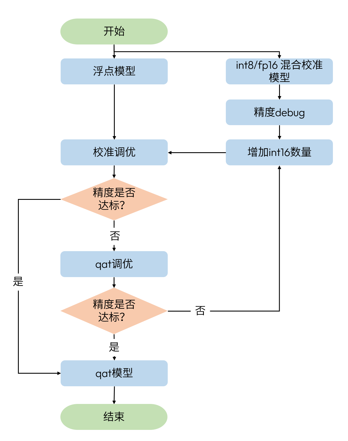
The following is an example in int8 / int16 / fp16 mixed precision tuning where the top 1 operator in int16 sensitivity is set to fp16, and the top 20% of int8 sensitivity is set to int16.

module_name_to_qconfig = {
    "op_1": get_qconfig(in_dtype=torch.float16, weight_dtype=torch.float16, out_dtype=torch.float16),
}

qat_model = prepare(
    model,
    example_inputs=example_input,
    qconfig_setter=(
        ModuleNameQconfigSetter(module_name_to_qconfig),
        sensitive_op_8bit_weight_16bit_act_calibration_setter(table, ratio=0.2),
        default_calibration_qconfig_setter,
    )
)
qat_model = prepare(
    model,
    example_inputs=example_input,
    qconfig_setter=(
        ModuleNameQconfigSetter(module_name_to_qconfig),
        sensitive_op_8bit_weight_16bit_act_qat_setter(table, ratio=0.2),
        default_qat_qconfig_setter,
    )
)

#J6P Mixed Precision Tuning

J6P has stronger floating-point capability and supports FP16 computation for non-gemm operators. In most cases, you only need to configure non-gemm operators as FP16, and then adjust the int8 / int16 ratio of gemm operators such as conv, convtranspose, linear, and matmul to get a quantized model that meets the accuracy target. For this reason, the main tuning path on this platform is usually more direct than on J6E/M. The tuning methods and accuracy tuning tool usage can be referenced directly from the earlier common sections, so they are not repeated here.

#Tuning Workflow

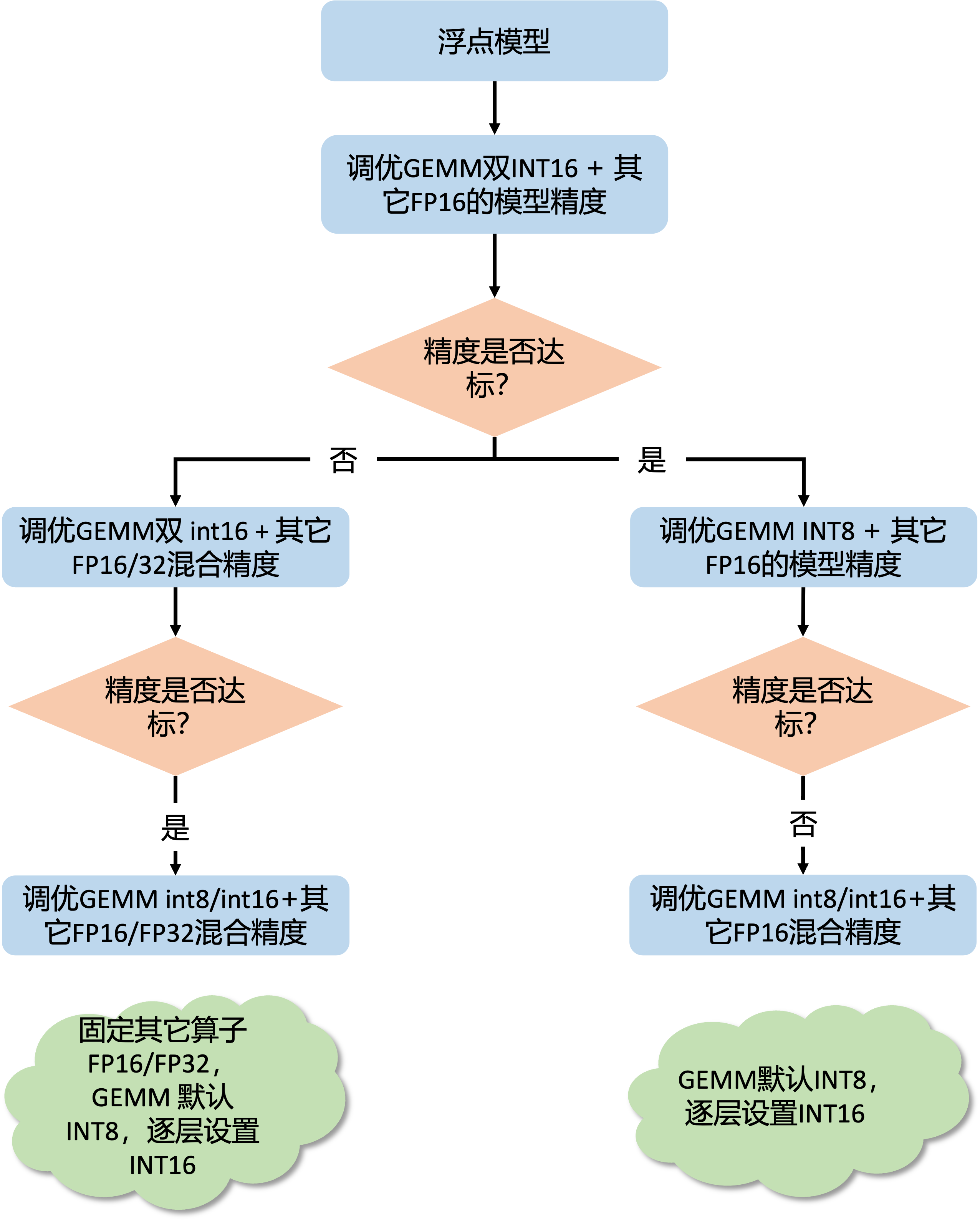
Consistent with the earlier common mixed precision workflow, J6P is also recommended to start from a relatively high-precision configuration. A common recommendation is to begin mixed precision tuning from a configuration where gemm operator inputs use dual int16 and all other operators use FP16.

1. After confirming that the configuration with gemm operator inputs as dual int16 and other operators as FP16 already meets the accuracy target, keep the other operators in FP16 and continue tuning gemm operator inputs with int8. If accuracy is still insufficient, continue with gemm operator input int8 / int16 mixed precision tuning, gradually increasing the proportion of int16 on top of the full int8 setting. At this stage, accuracy and performance still need to be balanced to find the best-performing configuration that also meets the accuracy target.

2. If the configuration with gemm operator inputs as dual int16 and other operators as FP16 still does not meet the accuracy target, keep gemm operator inputs as dual int16 and apply targeted handling to non-gemm operators as described below. Then on top of that, continue tuning gemm operator inputs with int8, keep the fp16 and targeted settings for the other operators fixed, and adjust the ratio of gemm operator input int16 in the same way as item 1.

#Tuning With Dual int16 Gemm Inputs and FP16 for Other Operators

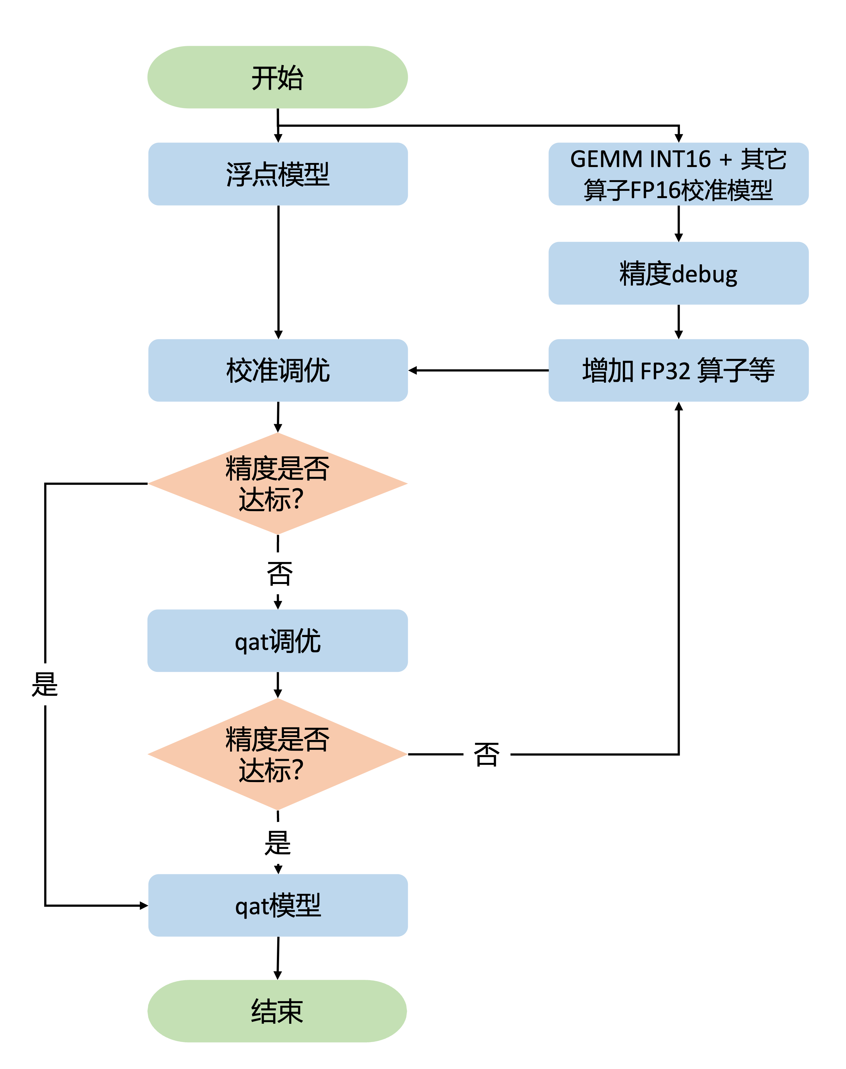
The QconfigSetter configuration is as follows:

from horizon_plugin_pytorch.quantization import prepare, PrepareMethod, get_qconfig
from horizon_plugin_pytorch.quantization.qconfig_setter import *

setter = QconfigSetter(
    reference_qconfig=get_qconfig(),
    templates=[
        ModuleNameTemplate({"": torch.float16}),  # Configure all operators with float16 output
        ConvDtypeTemplate(input_dtype=qint16, weight_dtype=qint16),  # Configure conv input and weight as int16
        MatmulDtypeTemplate(input_dtypes=qint16),  # Configure both matmul inputs as int16
    ],
)

qat_model = prepare(
    model,
    example_inputs=example_inputs,
    qconfig_setter=setter,
    method=PrepareMethod.JIT_STRIP,
)

If the current configuration still does not meet the accuracy target, you still need to continue judging it together with the series of debug results produced by the accuracy tuning tools. When looking at operators ranked high in sensitivity, two common cases usually appear:

1. Accuracy is still insufficient even with dual int16 gemm inputs. For gemm operators, dual int16 inputs can solve the vast majority of cases. If there are gemm operators whose inputs are already int16 but still rank high in input sensitivity, first consider whether fixed scale is needed for those inputs.

2. Accuracy is still insufficient for non-gemm operators in FP16. Compared with int16, FP16 supports a larger numeric range, but this comes at the cost of some numeric precision. The main cases identified so far where FP16 is not accurate enough are as follows.

• Coordinate-related computation, such as the grid input of gridsample. Coordinate precision affects sampling point selection, and even a small shift in the sampling point may have a large impact on the final result. So coordinate-related computation is recommended to use int16, and fixed scale can be set if necessary.

• Linear transform operators such as mul, where scaling can be inserted before and after the transform. A typical example is norm-like operators, where the intermediate mul output range becomes very large and may exceed the numeric range of FP16, causing truncation. In that case, it is recommended to scale the operator input and multiply it by a coefficient to reduce the input range. The framework already performs automatic scaling for FP16 configuration of layernorm. If similar cases appear elsewhere, the same scaling approach can also be considered.

• Nonlinear transform operators such as sigmoid. After scaling the input and output of such operators, the result usually cannot be restored equivalently to the original value before scaling. For example, after the input of sigmoid is scaled, the output of sigmoid cannot be restored to the corresponding value before input scaling. In that case, it is recommended to try FP32.

#Tuning With Gemm Inputs in int8/int16 and FP16 for Other Operators

Before tuning gemm inputs with int8/int16 and other operators with FP16, you should already have completed mixed precision tuning with gemm inputs as dual int16 and other operators as FP16. Next, reuse the verified configuration or adjustments from the previous stage, and continue accuracy debug on top of the configuration where gemm inputs use int8 and other operators use FP16. Then follow the method from the previous section and keep adjusting the ratio of int16 on gemm operators until the minimum int16 ratio that satisfies the accuracy requirement is found.

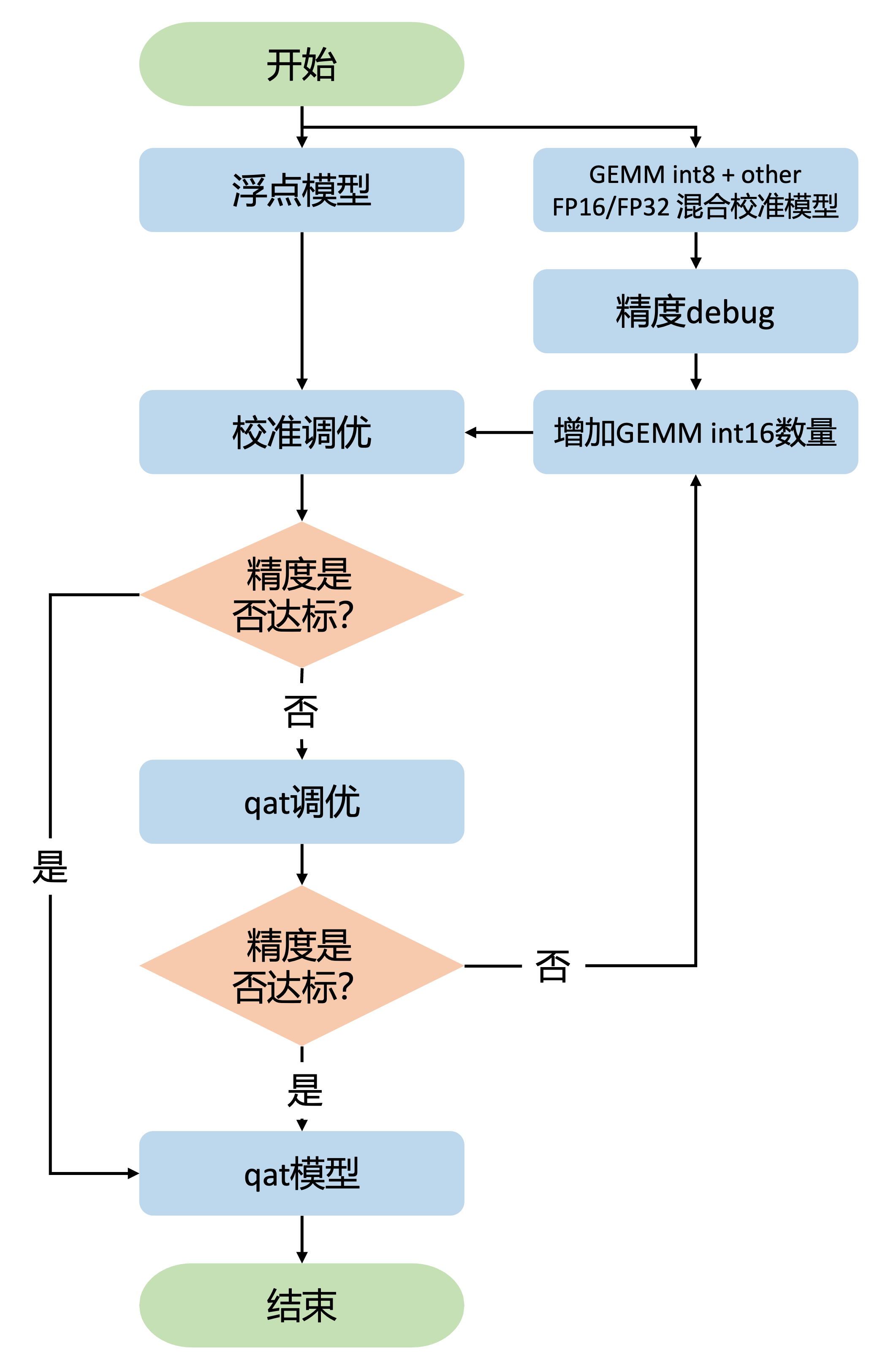
The QconfigSetter configuration is as follows:

from horizon_plugin_pytorch.quantization import prepare, PrepareMethod, get_qconfig
from horizon_plugin_pytorch.quantization.qconfig_setter import *

setter = QconfigSetter(
    reference_qconfig=get_qconfig(),
    templates=[
        ModuleNameTemplate({"": torch.float16}),  # Configure all operators with float16 output
        ConvDtypeTemplate(input_dtype=qint8, weight_dtype=qint8),  # Configure conv input and weight as int8
        MatmulDtypeTemplate(input_dtypes=qint8),  # Configure both matmul inputs as int8
            SensitivityTemplate(  # If highly sensitive feat or weight is configured as int8, change it to int16
                sensitive_table=...,
                topk_or_ratio=...,
            ),
    ],
)

qat_model = prepare(
    model,
    example_inputs=example_inputs,
    qconfig_setter=setter,
    method=PrepareMethod.JIT_STRIP,
)