#Model Calibration

In the quantization process, one key step is to determine the quantization parameters. Reasonable initial quantization parameters can significantly improve model accuracy and reduce the difficulty of subsequent QAT training.

After model transformation and floating-point training are completed, you can start Calibration. Calibration is the process of inserting Observers into the floating-point model, using a small amount of training data, and collecting data distributions at different positions during model forward, so as to determine more suitable quantization parameters.

• For some models, Calibration alone can already meet the accuracy target, so there is no need to continue with the more time-consuming QAT.

• Even if the accuracy after Calibration still does not meet the target, this step usually reduces the difficulty of later QAT training, shortens convergence time, and improves the final training accuracy.

#Overall Calibration Flow

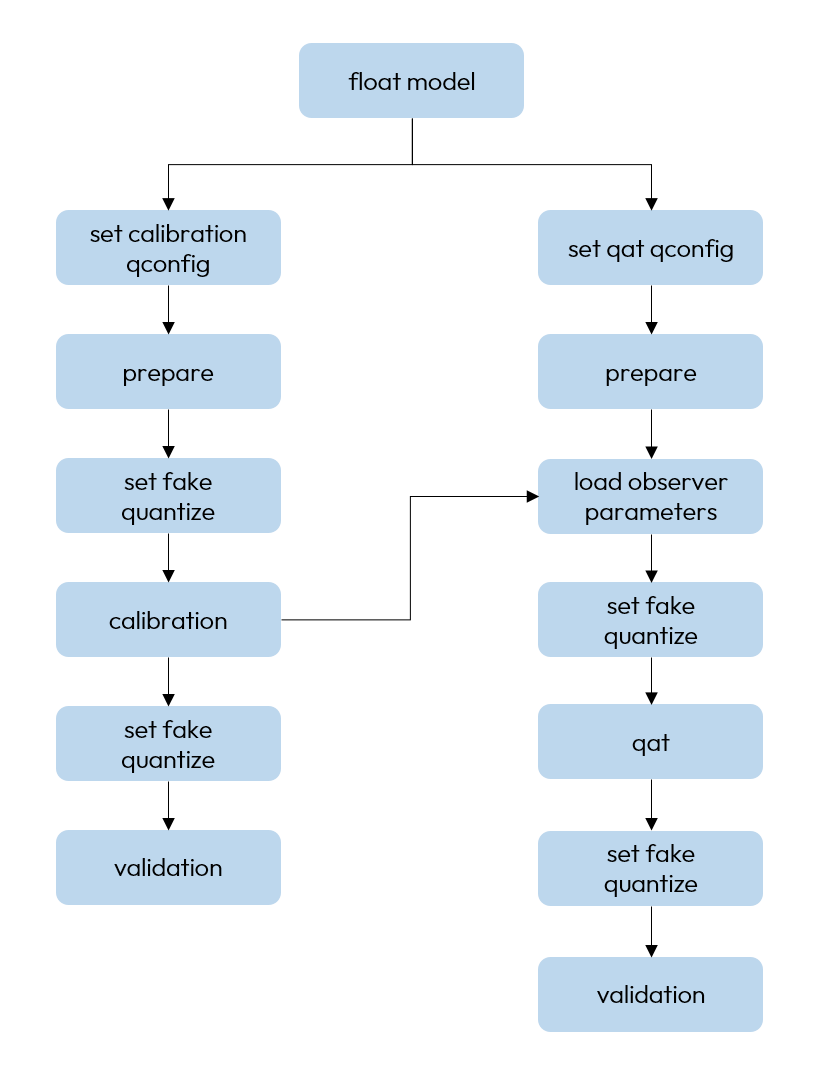
After Prepare is completed, the goal of Calibration is to use calibration data to collect tensor distributions at different positions in the model, so as to provide better initial quantization parameters for the subsequent quantization computation. The overall flow is shown below:

Before starting Calibration, you need to complete Build Floating-point Model, Build QConfig, and Prepare Description first. Below, we introduce the overall Calibration steps in the actual usage order.

1. Prepare the data used for Calibration and Validation first.

   In actual use, you will usually prepare one calib_data_loader for executing Calibration, and another eval_data_loader for evaluating the result after Calibration. For suggestions on how to choose the data, refer to the Calibration Data Preparation section below. The prepare_data_loaders(...) below is only a placeholder example, and you can replace it with the data preparation method used in your own project.

   # batch size used for Calibration
   calib_batch_size = 256
   
   # batch size used for Validation
   eval_batch_size = 256
   
   # amount of data used for Calibration, use inf to indicate all data
   num_examples = float("inf")
   
   calib_data_loader, eval_data_loader = prepare_data_loaders(
       data_path,
       calib_batch_size,
       eval_batch_size,
   )

   Here, calib_data_loader is used for executing Calibration, and eval_data_loader is used for evaluation after Calibration. If you currently only want to complete the main Calibration flow first, you can also prepare only the data needed for Calibration.

2. First set the model to eval, and then switch the fake quantize state to CALIBRATION, as shown below:

   from horizon_plugin_pytorch.quantization import FakeQuantState, set_fake_quantize
   
   calib_model.eval()
   set_fake_quantize(calib_model, FakeQuantState.CALIBRATION)

   fake quantize commonly has three states, which need to be switched before QAT, Calibration, and Validation, respectively.

   • CALIBRATION. Only collects the statistics of operator inputs and outputs.

   • QAT. Collects statistics and also performs fake quantization.

   • VALIDATION. Only performs fake quantization and no longer updates statistics.

   class FakeQuantState(Enum):
       QAT = "qat"
       CALIBRATION = "calibration"
       VALIDATION = "validation"

3. Execute Calibration. Feed the prepared calibration data into the model. The Observer will collect the relevant statistics during model forward. How the later quantization parameters are calculated depends on the Observer configured in qconfig and its search strategy. During Calibration, you usually only need to run forward and do not need backward. An example is shown below:

   import torch
   
   with torch.no_grad():
       for batch in calib_data_loader:
           image = batch[0].to(device)
           calib_model(image)

   If your dataloader directly returns the model input, you can also feed batch directly into the model for forward.

4. After Calibration is completed, set the model to eval and switch the fake quantize state to VALIDATION, so that you can evaluate the current Calibration result.

   from horizon_plugin_pytorch.quantization import FakeQuantState, set_fake_quantize
   
   calib_model.eval()
   set_fake_quantize(calib_model, FakeQuantState.VALIDATION)

   If you already have an evaluation function, you can directly use eval_data_loader to evaluate calib_model, for example:

   top1, top5 = evaluate(calib_model, eval_data_loader, device)

5. Verify the Calibration result. If the result already meets your requirement, you can directly convert the model to a fixed-point model, or continue with subsequent quantization aware training on top of it. If the result does not meet your requirement, refer to the section Recommendations When Calibration Does Not Meet Expectations.

#Calibration Data Preparation

The previous workflow section explains the overall Calibration flow. Here we further explain what you should pay attention to when preparing calibration data in actual use.

The Calibration result is highly related to the calibration data distribution. In actual use, we recommend that you first pay attention to the following points:

1. More Calibration data is not always better. After the data size reaches a certain scale, the gain from adding more data becomes limited. If the training set is small, you can use all of it for Calibration. If the training set is large, you can choose a suitable subset according to Calibration cost. It is recommended to run at least 10 to 100 steps of Calibration.

2. Calibration data should cover the typical input distribution of the model as much as possible, and all deployment scenarios should be included. Otherwise, Calibration may become biased and even cause distorted quantization parameters. For example, if the application scenarios include daytime, nighttime, urban roads, highways, curves, and straight roads, the calibration data should cover all of them as much as possible.

3. For image tasks, it is recommended to use inference-stage preprocessing together with training data for Calibration whenever possible.

4. When using image augmentation, you can use relatively mild augmentation such as horizontal flip. It is not recommended to use augmentation such as mosaic, which significantly changes the data distribution.

#Calibration Algorithms and Search Strategies

After completing the basic Calibration flow and preparing the calibration data, the next thing to pay attention to is how the quantization parameters are actually calculated. This part is mainly determined by the Observer configured in qconfig and its corresponding scale search strategy.

In the previous workflow, the Observer has already been inserted into the model through qconfig. When forward is actually executed during Calibration, the Observer collects tensor distributions and then calculates the scales and other parameters needed for quantization. Different Observers use different statistics and search strategies, so the final Calibration result may also differ. Therefore, in the Calibration stage, we focus more on how they work during calibration and what differences different strategies may introduce.

We recommend using HistogramObserver in Calibration. It collects the overall distribution of the calibration set and automatically chooses a more suitable scale together with the search strategy. Compared with some other Observers that usually use per-frame computation plus moving average, this approach is often more stable in practice. From actual usage experience, HistogramObserver is also generally a better default choice in terms of both result stability and accuracy performance.

The common search methods are as follows:

After Calibration is completed with the default search strategy, if the accuracy still does not meet expectations, you can use HistogramObserver.reset_scale to recalculate the scale with other strategies, without running Calibration again. The reference definition is shown below:

class HistogramObserver:
    @classmethod
    def reset_scale(
        cls,
        model,
        method,
        method_kwargs=None,
        prefix=None,
        dtype=None,
    ):
        """Reset scales in model by specified method.

        Args:
            model (torch.nn.Module): Model calibrated with HistogramObserver.
            method (str): Chosen from ('mse', 'percentile').
            method_kwargs (Dict, optional): For 'percentile' method, user can set `{'percentile': 0.0~1.0}` to control the proportion of numerical values included in the quantization interval. Defaults to None.
            prefix (Tuple[str], optional): Only reset scale in specified scopes. Defaults to None.
            dtype (_type_, optional): Only reset scale of specified quant dtype. Defaults to None.
        """

#Reusing Calibration Results when Adjusting Quantization dtype

In the previous section on calibration algorithms and search strategies, we recommend using HistogramObserver for calibration. Unlike some Observers in earlier versions that use a per-frame statistics + moving-average strategy, histogram calibration collects the global distribution over the entire calibration set and computes scale from that distribution.

Because scale is computed from global information, after you complete one Calibration run, you can adjust the quantization dtype of certain nodes based on subsequent quantization analysis results and recalculate the corresponding scales from the statistics collected during calibration without re-running the calibration procedure. For this purpose, we provide the load_calib_state_dict API. When loading a Calibration checkpoint into a QAT or Validation model, it recalculates scale according to the actual dtype of fake-quant nodes.

#Supported dtype transition scope

Because float16 requires global min/max statistics that HistogramObserver does not yet cover, load_calib_state_dict only supports the following dtype transitions:

#Recommended workflow

Overall approach: Complete Calibration with a relatively relaxed qconfig and save state_dict, then prepare the target model according to analysis results, and finally inject calibration results with load_calib_state_dict.

1. Perform the first prepare on the floating-point model and complete Calibration. During Calibration, it is recommended to disable Conv + add fuse in QconfigSetter (conv input dtype is not yet finalized at this stage; if conv input is later changed to qint16, fuse may no longer be possible). Skipping fuse during Calibration is compatible with both subsequent fuse and no-fuse cases.

2. Save calib_state_dict = calib_model.state_dict().

3. On top of the qconfig used for Calibration, adjust the template according to sensitivity analysis and other results (for example, promote some layers from qint8 to qint16), run prepare again on another copy of the floating-point model, and obtain qat_model or predict_model for evaluation.

4. Call load_calib_state_dict to load Calibration results, then proceed to Validation or QAT.

import copy

from horizon_plugin_pytorch.quantization import FakeQuantState, load_calib_state_dict, prepare, set_fake_quantize
from horizon_plugin_pytorch.quantization.qconfig_setter import (
    FuseConvAddTemplate,
    OutputHighPrecisionTemplate,
    QconfigSetter,
)

# 1. Calibration model: disable Conv+add fuse and complete calibration
calib_model = prepare(
    copy.deepcopy(model),
    example_inputs,
    qconfig_setter=QconfigSetter(
        ...,
        optimize_templates_kwargs={
            FuseConvAddTemplate: {
                "enabled": False,
            },
            OutputHighPrecisionTemplate: {
                "enabled": False,
            },
        },
    ),
)
# ... Calibration steps omitted

calib_state_dict = calib_model.state_dict()

# 2. Re-prepare the target model after adjusting qconfig based on quantization analysis
qat_model = prepare(
    copy.deepcopy(model),
    example_inputs,
    qconfig_setter=...,  # Add qint8->qint16 changes on top of the calib configuration
)

# 3. Load calib results; scales are recalculated according to the model's actual dtype
load_calib_state_dict(qat_model, calib_state_dict)

# 4. Evaluate or continue with QAT
qat_model.eval()
set_fake_quantize(qat_model, FakeQuantState.VALIDATION)
evaluate(qat_model, eval_data_loader, device)

When entering Quantized Awareness Training, it is also recommended to use load_calib_state_dict(qat_model, calib_state_dict) instead of directly calling qat_model.load_state_dict(calib_model.state_dict()), so that scale can still be restored correctly when the QAT qconfig is not fully consistent with the Calibration stage.

#Calibration Strategies on Different Platforms

The recommended starting point is not exactly the same on different platforms. During Calibration, it is also recommended to adopt different strategies according to platform characteristics.

#J6E/M/B

For J6E/M/B, it is recommended to first use full int16 configuration to see the upper bound of accuracy, and then move back to mixed int8 + int16 precision.

• If the model is being connected to QAT for the first time, or if the current accuracy issue is relatively complicated, it is recommended to first validate the upper bound with a full int16 template.

• If the result under full int16 improves significantly, then gradually roll back to mixed int8 + int16 precision to balance accuracy and performance.

• If the result is still poor even under full int16, it is usually not recommended to directly enter QAT. Instead, you should first revisit the model structure, calibration data, and fix scale configuration, and then use sensitivity analysis if necessary.

#J6H/P

For J6H/P, it is recommended to make use of the stronger floating-point capability of the platform and start from the idea of global fp16 + GEMM int8 / int16.

• A common starting point is global fp16, while configuring GEMM-type operators such as Conv / Matmul / Linear as int8.

• If the basic configuration still does not meet the requirement, then use sensitivity results to raise key GEMM operators to int16.

• For vector-type computation, fp16 usually helps reduce the difficulty of quantization tuning. In actual use, you also need to pay attention to issues such as fp16 range overflow, mixed int16 / fp16 usage, and output type changes.

For more detailed platform differences, refer to Platform Differences.

#Calibration Result Verification Recommendations

After Calibration is completed, we recommend that you judge the next step according to the following guideline first:

#Recommendations When Calibration Does Not Meet Expectations

When the accuracy after Calibration does not meet expectations, we recommend that you continue to Precision Tuning Guide and use the detailed usage, applicable scenarios, and result interpretation of the following methods to locate the issue:

• Staged quantization. Quantization is gradually introduced by model stages, submodules, or local segments, so that you can observe where the error begins to increase significantly and narrow down the problem scope first.

• Histogram analysis. Observe the input/output or activation distributions of key layers to help determine whether there are truncation, saturation, abnormal scales, distorted distributions, or long-tail issues.

• Sensitivity analysis. Identify operators that have a larger impact on the model output according to quantization sensitivity results, and use this as the basis for raising the quantization precision of related operators.

These methods have different roles. Staged quantization is more suitable for narrowing down the problem scope first. Histogram analysis is more suitable for further judging whether the scale of key layers is abnormal. Sensitivity analysis is more suitable for determining where higher precision should be added.

If you find that quantized.bc / hbm degrades significantly after Calibration, it is also recommended to first continue to Deployment Consistency Analysis for further investigation.